. 1999 May 15;19(10):4046-64.
doi: 10.1523/JNEUROSCI.19-10-04046.1999.

Functional micro-organization of primary visual cortex: receptive field analysis of nearby neurons

Affiliations

Functional micro-organization of primary visual cortex: receptive field analysis of nearby neurons

G C DeAngelis et al. J Neurosci. .

Abstract

It is well established that multiple stimulus dimensions (e.g., orientation and spatial frequency) are mapped onto the surface of striate cortex. However, the detailed organization of neurons within a local region of striate cortex remains unclear. Within a vertical column, do all neurons have the same response selectivities? And if not, how do they most commonly differ and why? To address these questions, we recorded from nearby pairs of simple cells and made detailed spatiotemporal maps of their receptive fields. From these maps, we extracted and analyzed a variety of response metrics. Our results provide new insights into the local organization of striate cortex. First, we show that nearby neurons seldom have very similar receptive fields, when these fields are characterized in space and time. Thus, there may be less redundancy within a column than previously thought. Moreover, we show that correlated discharge increases with receptive field similarity; thus, the local dissimilarity between neurons may allow for noise reduction by response pooling. Second, we show that several response variables are clustered within striate cortex, including some that have not received much attention such as response latency and temporal frequency. We also demonstrate that other parameters are not clustered, including the spatial phase (or symmetry) of the receptive field. Third, we show that spatial phase is the single parameter that accounts for most of the difference between receptive fields of nearby neurons. We consider the implications of this local diversity of spatial phase for population coding and construction of higher-order receptive fields.


Figures

Fig. 1.
Fig. 1.
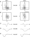
Spatiotemporal RF profiles for a pair of simple cells recorded simultaneously from the same microelectrode. Each RF profile describes the sensitivity of the cell to luminance increments and decrements as a function of space (X,Y) and time (T). For each neuron, four spatial (X–Y) cross sections, taken at equally spaced time increments, are shown (top). In addition, each RF profile is summarized as an X–T plot (bottom) by integrating the X–Y–T data along the Y-axis, which is approximately parallel to the preferred orientation of each cell. Each X–Y orX–T profile is plotted as an isoamplitude contour map, in which solid contours represent responses to luminance increments, and dashed contours denote responses to luminance decrements. For additional details concerning the construction of RF profiles, see our previous papers (DeAngelis et al., 1993a, 1995a; Ohzawa et al., 1996). For this pair of simple cells, theX–Y–T SI is 0.17 (see Results for details).
Fig. 2.
Fig. 2.
Receptive field cross sections and their corresponding SIs are shown for the same pair of simple cells depicted in Figure 1. A, X–T profiles. The similarity index computed in the X–T plane is SIX–T = 0.26. B,XY cross sections taken atT = 60 msec. SIX–Y = 0.23.C, One-dimensional spatial cross sections taken parallel to the X-axis (i.e., perpendicular to the preferred orientation axis of the cells). Each X cross section was taken at T = 60 msec, as shown by thehorizontal lines through the X–Tprofiles in A. The SIX is 0.33, reflecting the fact that there is a clear difference in spatial phase betweenX profiles for the two cells. D, One-dimensional spatial cross sections taken parallel to theY-axis. The X-coordinate for eachY cross section is shown by the vertical lines through the XY profiles in B; T = 60 msec. SIY is 0.96, indicating that the Y cross sections for the two cells are quite similar. E, Temporal cross sections are shown. Vertical lines through theXT data in A give theX values at which these cross sections were obtained. Note that the two temporal profiles have a similar shape, resulting in an SIT value of 0.97.
Fig. 3.
Fig. 3.
Distributions of similarity indices for populations of simple-cell pairs from kittens (open bars) and adult cats (filled bars). All pairs of neurons were recorded simultaneously from a single microelectrode. Each histogram gives the distribution of SI for a different cross section through the spatiotemporal RF profile, as illustrated in Figure 2. Panels A,C, and E show data for pairs of neurons (n = 45 pairs for adults; n = 21 for kittens) for which RFs were mapped in either one or two spatial dimensions (see Materials and Methods). PanelsB, D, and Fshow data for a subpopulation of pairs (n = 29 pairs for adults; n = 4 for kittens) for which fullX–Y–T profiles were obtained. The Y,XY, and X–Y–T cross sections are defined only for this latter group of neurons.
Fig. 4.
Fig. 4.
Quantitative summary of RF similarity indices as a function of the dimensionality of the RF cross section. The height of each bar gives the median absolute value of SI for the populations of cell pairs in Figure 3 (i.e., each histogram in Fig. 3 is folded about the SI = 0 axis, and the median value of the resultant distribution is computed). Open and filled bars denote population data obtained from kittens and adult cats, respectively.
Fig. 5.
Fig. 5.
Spatiotemporal RF profiles and cross-correlograms for two pairs of simple cells. A, X–Tprofiles for a pair of simple cells from a 4-week-old kitten that have similar RFs. B, Raw cross-correlogram for the same pair of cells as in A. The correlogram was constructed from spike trains recorded during the reverse-correlation mapping experiment. C, X–T profiles for a pair of simple cells recorded from an adult cat. D, Raw correlogram for the pair of neurons in C. Note that the small notch just to the left of zero is an artifact caused by the fact that the two neurons were recorded simultaneously from a single microelectrode.
Fig. 6.
Fig. 6.
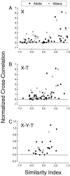
Relationship between correlated discharge and receptive field similarity. Each graph plots normalized cross-correlation (see Results for details) against the similarity index computed from a different RF cross section:X (A), X–T(B), and X–Y–T(C). Filled circles show data from adult cats; open circles show data from 4-week-old kittens. Note that the magnitude of correlated discharge is larger in the SIX and SIX–T distributions. This is because these distributions include 1-D reverse correlation runs in which elongated bars are used. These bars are a more effective stimulus than the smaller bars used in 2-D runs, and therefore elicit both stronger individual responses and stronger correlated responses.
Fig. 7.
Fig. 7.
Examples of simple cell pairs that have SI values near zero in the X–T domain. A, TheX–T profiles of this pair of simple cells are similar, except for a spatial phase difference of ∼90° (i.e., spatial quadrature); SIX–T = 0.11. B, The two members of this pair of cells prefer opposite directions of motion, as evidenced by the difference in the space–time orientation of their subregions. SIX–T for this pair is −0.13.
Fig. 8.
Fig. 8.
Spatiotemporal RF model used to fit theX–T profiles of simple cells in this study. In this model, a spatiotemporally inseparable RF (bottom) is constructed as the weighted sum of two separable RFs. The two separable subunits are identical except for a 90° difference in their spatial and temporal phases (see Results for details). As the weight, α, on the second subunit increases from 0.0 to 1.0, the resultant model RF changes from space–time separable to strongly inseparable.G1(X),H1(T),G2(X),H2(T), andR(X,T) denote the quantities referred to in Equation 2 (see Results).
Fig. 9.
Fig. 9.
Representative fits of the spatiotemporal RF model to X–T profiles for three pairs of simple cells (AC). For each neuron, the left panel shows the measured RF profile, the center panel shows the best fit of the model depicted in Figure 8, and the right panel shows the error profile (i.e., the difference between the data and the fit). Note that all three contour maps for a given cell are plotted on the same response scale. See Results for additional details.
Fig. 10.
Fig. 10.
Distribution of the fractional error metric used to quantify the quality of fits of the RF model to data. Fractional error of the fit is defined as the sum of squares of the error profile (Fig. 9A, right) divided by the sum of squares of the raw data (Fig. 9A,left). Filled and open barsdenote data from adult cats and kittens, respectively.
Fig. 11.
Fig. 11.
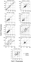
Summary of pairwise correlations in various RF parameters. Each panel here is a scatter plot in which the parameter value for one cell (cell 1) is plotted on the horizontal axis, and the value for a simultaneously recorded neuron (cell 2) is plotted on the vertical axis. Filled and open circlesrepresent data from adult cats (n = 45 pairs) and kittens (n = 21 pairs), respectively.A, Preferred orientation shows strong clustering, with most data points distributed tightly around the diagonal line of unity slope. Note that these data were obtained from responses to drifting grating stimuli, whereas the remaining data in this figure were extracted from fits to the X–T profiles.B, Peak response latency,t0, shows modest clustering. Note that t0 here is expressed in units of milliseconds, whereas T0 in the model (Eq.4) is defined in skewed time coordinates. C, Scatter plot of RF width, w, as defined in Equation 3.D, Scatter plot of response duration, D. D is defined as the width of the temporal response envelope at a criterion amplitude of 1/e (or 0.37 of the peak amplitude), and is expressed in units of milliseconds. Note that, althoughD is determined by the parameter c in Equation 4, c is not used directly here because it is defined in skewed time coordinates. E, Preferred spatial frequency, sf (defined as in Eq. 3), shows pronounced clustering. F, Scatter plot of preferred temporal frequency, tf. Note thattf here is expressed in units of hertz.G, Scatter plot of the spatial phase of the receptive field, P. Because P is a circular variable, the largest possible difference in phase between two neurons is 180°. Thus, all of the data points shown here are constrained to fall within the pair of dashed lines. H, Distribution of temporal phase, Q. These data are plotted on the same axes as those of panel G to facilitate comparison. I, Scatter plot for the linear direction selectivity index, α. Positive and negative values of α correspond to opposite directions of motion, and larger values of  α  correspond to stronger direction selectivity. Thus, data points in the top right quadrant denote pairs of neurons with the same direction preference, whereas points in the top left or bottom right quadrants indicate pairs with opposite preferred directions of motion.
Fig. 12.
Fig. 12.
Quantitative analysis of clustering for the spatial and temporal response parameters of Figure 11.Filled and unfilled bars correspond to data from adult cats and kittens, respectively. Each bar gives the clustering index (see Results for details) for a particular response parameter. Asterisks above some bars indicate that the associated clustering index is significantly >1.0 (**p < 0.01; *p < 0.05).OR, Preferred orientation; w, RF width;sf, preferred spatial frequency;t0, peak response latency;D, response duration; tf, preferred temporal frequency; P, spatial phase; Q, temporal phase; and α, direction selectivity index.
Fig. 13.
Fig. 13.
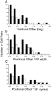
Analysis of receptive-field overlap.A, Distribution of positional offsets between RFs of simultaneously recorded pairs of simple cells. Filledand unfilled bars show data from adult cats and kittens, respectively. Positional offset is defined as the spatial displacement (along the X-axis) between the centers of the spatial envelopes of two RFs [i.e., abs(x0Ax0B)]. B, Distribution of positional offsets normalized by the average RF width of the two neurons [i.e., abs(x0Ax0B)/(0.5 (wA +wB)], where the subscriptsA and B denote the two members of a pair of neurons. C, Distribution of positional offsets expressed as a number of cycles at the preferred spatial frequency of the cells. The offset in cycles is computed as abs(x0Ax0B) (0.5 (sfA +sfB), wheresfA and sfB are the preferred spatial frequencies for the two neurons of each pair.
Fig. 14.
Fig. 14.
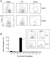
Simultaneous-fitting analysis for quantifying the contribution of various RF parameters to the overall difference in structure between a pair of RFs. A, Data, fit, and error profiles for a pair of simple cells from an adult cat that differ predominantly in terms of spatial phase (i.e., an antiphase pair). TheX–T data for both neurons was fit simultaneously with the RF model of Equations 2-4 (22 parameter fit). B, Summary of changes in the overall error of the fit, expressed as percent error elevation, when different parameters of the RF model are forced to have a common value for the two neurons. Because one parameter is common to the pair, the resulting fit has 21 parameters. The inset shows the best fit of the model, along with the resulting error profiles, when spatial phase is the common parameter. Note that the error profiles are larger and substantially more structured than those in panel A. Parameters of the model are denoted as follows: x0, RF center position; w, RF width; sf, preferred spatial frequency; P, spatial phase;t0, peak response latency;c, temporal envelope width; β, temporal skewing factor; tf, preferred temporal frequency;Q, temporal phase; and α, direction selectivity index.
Fig. 15.
Fig. 15.
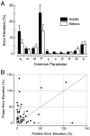
Summary of the relative contributions of various model parameters to the overall difference in structure between pairs of RFs. A, Mean error elevation (+1 SE) is shown for each RF parameter. Filled and open barsshow data from adult cats and kittens, respectively. Parameter notations are as described in Figure 14B.B, Phase error elevation is plotted against position error elevation for all pairs of simple cells from adults (filled circles) and kittens (open circles).
Fig. 16.
Fig. 16.
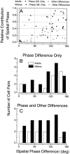
Analysis of spatial phase differences between pairs of simple cells. A, The relative contribution of spatial phase to the overall difference in structure between pairs of RFs is plotted as a function of the spatial phase difference between each pair of neurons. Relative contribution of phase is defined as the percent error elevation caused by spatial phase divided by the total percent error elevation caused by all parameters. If the percent error elevation caused by spatial phase is large, and that caused by all other parameters is small (Fig. 14B), then the relative contribution of spatial phase will approach 1.0.Circles and diamonds denote data from adult cats and kittens, respectively. Filled symbolscorrespond to pairs of neurons for which the relative contribution of all RF parameters, other than spatial phase, does not exceed 0.2. The remaining pairs of neurons are denoted by open symbols.B, Histogram showing the distribution of spatial phase differences for pairs of simple cells that differ primarily in terms of spatial phase. Cell pairs included in this distribution are those represented by filled symbols in panel A.C, Distribution of spatial phase differences for pairs of simple cells that have a substantial relative contribution from parameters other than spatial phase (these data correspond to theopen symbols in panel A).
Fig. 17.
Fig. 17.
Receptive field profiles for a pair of binocular simple cells (KD655R39). Top row, X–Tprofiles and X cross sections, as measured through both the left eye and the right eye. This cell has an interocular phase difference of 45° (Table 1) and a preferred orientation that is 27° from vertical. Bottom row, RF profiles measured through the left and right eyes for a second simple cell, recorded simultaneously. This neuron has an interocular phase difference of 126° and a preferred orientation that is 18° from vertical.

Similar articles

Cited by

References

    1. Adelson EH, Bergen JR. Spatiotemporal energy models for the perception of motion. J Opt Soc Am A. 1985;2:284–299. - PubMed
    1. Albrecht DG, Geisler WS. Motion selectivity and the contrast-response function of simple cells in the visual cortex. Vis Neurosci. 1991;7:531–546. - PubMed
    1. Bartfeld E, Grinvald A. Relationships between orientation-preference pinwheels, cytochrome oxidase blobs, and ocular-dominance columns in primate striate cortex. Proc Natl Acad Sci USA. 1992;89:11905–11909. - PMC - PubMed
    1. Berardi N, Bisti S, Cattaneo A, Fiorentini A, Maffei L. Correlation between the preferred orientation and spatial frequency of neurones in visual areas 17 and 18 of the cat. J Physiol (Lond) 1982;323:603–618. - PMC - PubMed
    1. Berman NE, Wilkes ME, Payne BR. Organization of orientation and direction selectivity in areas 17 and 18 of cat cerebral cortex. J Neurophysiol. 1987;58:676–699. - PubMed

Publication types

LinkOut - more resources