State-dependent inactivation of the alpha1G T-type calcium channel

Abstract

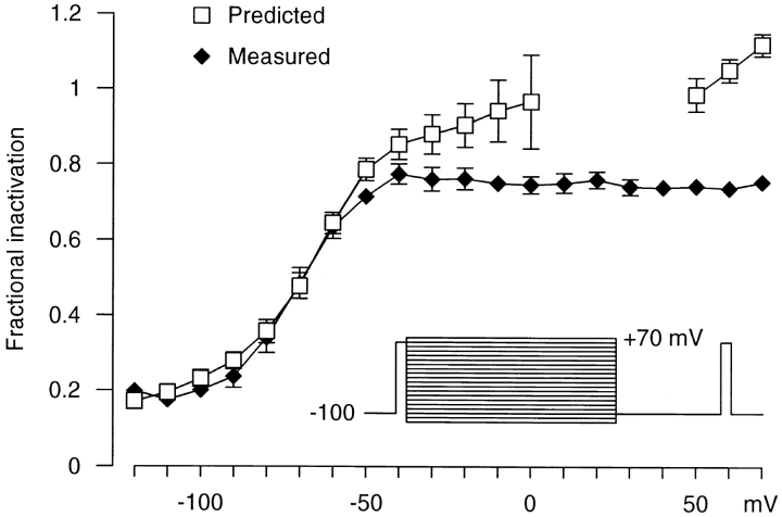
We have examined the kinetics of whole-cell T-current in HEK 293 cells stably expressing the alpha1G channel, with symmetrical Na(+)(i) and Na(+)(o) and 2 mM Ca(2+)(o). After brief strong depolarization to activate the channels (2 ms at +60 mV; holding potential -100 mV), currents relaxed exponentially at all voltages. The time constant of the relaxation was exponentially voltage dependent from -120 to -70 mV (e-fold for 31 mV; tau = 2.5 ms at -100 mV), but tau = 12-17 ms from-40 to +60 mV. This suggests a mixture of voltage-dependent deactivation (dominating at very negative voltages) and nearly voltage-independent inactivation. Inactivation measured by test pulses following that protocol was consistent with open-state inactivation. During depolarizations lasting 100-300 ms, inactivation was strong but incomplete (approximately 98%). Inactivation was also produced by long, weak depolarizations (tau = 220 ms at -80 mV; V(1/2) = -82 mV), which could not be explained by voltage-independent inactivation exclusively from the open state. Recovery from inactivation was exponential and fast (tau = 85 ms at -100 mV), but weakly voltage dependent. Recovery was similar after 60-ms steps to -20 mV or 600-ms steps to -70 mV, suggesting rapid equilibration of open- and closed-state inactivation. There was little current at -100 mV during recovery from inactivation, consistent with </=8% of the channels recovering through the open state. The results are well described by a kinetic model where inactivation is allosterically coupled to the movement of the first three voltage sensors to activate. One consequence of state-dependent inactivation is that alpha1G channels continue to inactivate after repolarization, primarily from the open state, which leads to cumulative inactivation during repetitive pulses.

Figure 7

Voltage dependence of steady state inactivation. Steps lasting 1 s to the indicated voltages were followed by 5-ms test pulses to −20 mV. The protocol was run either with no preceding depolarization (for inactivation) or immediately after a 60-ms step to −20 mV (for recovery). For the recovery protocol, the values are the ratio of current in the test pulse to the current during the 60-ms prepulse, measured at comparable times. For the inactivation protocol, currents were normalized to the value at −100 mV (i.e., with no prepulse). Test pulses (with no prepulse) were given before and after the rest of the protocol, to control for rundown or accumulation of inactivation. The smooth curves are fits to a Boltzmann relation, with (inactivation) and (recovery). Cell a8n02, 1 kHz analogue antialias filtering.

Figure 1

Current–voltage relations for α1G channels. (A) Sample current records, with 5 kHz Gaussian filtering, from cell e8612. (B) Current–voltage relations averaged from 12 cells, measured at the point of peak current at each voltage.

Figure 2

Envelope test for isolation of α1G currents. Depolarizations of variable duration were given to +60 mV (above) or −20 mV (below). The records shown lasted 2, 5, 10, 20, 50, and 100 ms. The peak amplitudes of the tail currents after repolarization for those records (and for steps lasting 0.2, 0.5, and 1 ms) were scaled to match the currents during depolarization, and are shown as open squares superimposed on the records. Cell a8612, 3 kHz Gaussian filtering.

Figure 3

Instantaneous current–voltage relations for α1G channels. (A) Sample current records, with 5 kHz Gaussian filtering, from cell e8612. The initial step to +60 mV lasted 2 ms. Records are shown for repolarizations in 20-mV increments. 2-ms test pulses to +60 mV were given at the end of the protocol, 20-ms after repolarization to −100 mV, to assess inactivation (not shown; see Fig. 11 below). (B) Instantaneous current–voltage relations, measured from the protocol of A, averaged from eight cells. Currents were measured at the peak of the tail current in each cell, which varied from 0.3 to 0.5 ms in these cells.

Figure 4

Activation of α1G channels. (A) Activation curve, from current ratios: the peak current recorded during depolarization directly to the indicated voltage (the protocol of Fig. 1), divided by the instantaneous current recorded after repolarization from a 2-ms step to +60 mV (the protocol of Fig. 3). Data are not shown for voltages near the reversal potential. . The smooth curve is a fit to a Boltzmann functions: mV, e-fold for 9.4 mV, amplitude 0.80. (B) Time to peak, for the protocol of Fig. 1, .

Figure 5

Time course of inactivation and deactivation. (A) Time constants are from single exponential fits, from two protocols. The diamonds are for currents recorded during direct depolarizations (the protocol of Fig. 1), with the fit beginning well after the point of peak inward current, and ending at 60 or 120 ms. The squares are for currents recorded after repolarization from +60 mV (the protocol of Fig. 3), fitted from 0.4–0.6 ms after repolarization to the end of the 40-ms steps. Data are from the same eight cells as Fig. 3 B. (B) Deactivation kinetics at strongly hyperpolarized voltages. Voltage steps were in 15-mV increments, from −90 to −150 mV. The records are from cell a8o29, with 5 kHz Gaussian filtering. The inset shows the time constants, which changed e-fold for 32.8 ± 0.4 mV .

Figure 6

Time course of inactivation and recovery. (A) Effect of prepulses of variable voltage and duration on the current evoked by a test pulse to −20 mV. The currents were normalized to that observed during a test pulse given alone (with no prepulse). The smooth curves are exponential functions, with time constants of 202 ms at −80 mV, and 210 ms at −70 mV. (B) The time course of recovery from inactivation, after 60-ms pulses to −20 mV. The values are the current during the test pulse to −20 mV, divided by the current at the corresponding time in the 60-ms prepulse. Time constants for recovery were 86 ms at −120 mV, 74 ms at −100 mV, and 175 ms at −80 mV. (C) The protocol for recovery from inactivation. Records (analogue filtering at 1 kHz) are shown for recovery at the holding potential of −100 mV, with recovery intervals of 8, 20, 40, 80, and 200 ms. All data in this figure are from cell a8612.

Figure 8

Test for window current. (A) Incomplete inactivation after 120-ms depolarizations. Tail currents at −100 mV were fitted to a single exponential (plus a constant) beginning 0.6–0.8 ms after repolarization from the voltages indicated (protocol of Fig. 1, except voltage steps lasted 120 ms). P _O,r was calculated by dividing the initial tail current amplitude (sum of the exponentially decaying component, plus the constant) by the instantaneous current at −100 mV after a 2-ms depolarization to +60 mV (the protocol of Fig. 3). Each symbol is a different cell , and the line is drawn through the mean values. (B) Incomplete inactivation for 300-ms depolarizations to −20 mV. The records are the averaged currents from four depolarizations, in each of five cells. The inset shows the current at the end of the step and the tail current, at a 10× higher amplification. 1 kHz Gaussian filter.

Figure 10

Recovery from closed-state inactivation. In this cell, a 600-ms step to −70 mV produced a small inward current , but a subsequent 10-ms test pulse to −20 mV demonstrated 40% inactivation (compared with 8% predicted open-state inactivation). The main figure shows the time course of recovery from inactivation at −100 mV, fitted to an exponential function with . Currents were measured during the steps to −20 mV, and were normalized to the current recorded during test pulses to −20 mV (with no prepulse to −70 mV) given after the protocol. The inset shows records for recovery intervals of 25, 50, 100, 250, 500, and 1,000 ms (cell d8o28, 500 Hz Gaussian filter). In this cell, the peak P _O,r and the amount of inactivation at −70 mV were both less than typically observed (compare with Fig. 6, Fig. 7, and Fig. 9).

Figure 9

Test for closed-state inactivation. Voltage steps to −70 mV (A) or −80 mV (B) for the indicated duration were immediately followed by 5-ms test pulses to −20 mV. Inactivation measured from the test pulses (diamonds) is compared with the expected open-state inactivation (squares) calculated from the integrated current during the step to −70 mV (). (A), (B).

Figure 12

Cumulative inactivation. (A) The upper panel is two superimposed current records, a single 50-ms depolarization to −20 mV, and four steps to −20 mV for 5 ms each, separated by 10-ms intervals at −100 mV. The lower panel is the predicted open-state inactivation for the four-pulse protocol. Cell a8612, 2 kHz Gaussian filter. (B) Inactivation during a train of four action potential–like depolarizations. Cell e8612, 5 kHz Gaussian filter. The voltage command (shown below) was simulated from the Hodgkin-Huxley (1952b) model for the squid axon, modified to allow spontaneous 50-Hz repetitive firing by shifting the voltage dependence of the “m” gate by 2 mV to more negative voltages. The action potentials were scaled to an initial voltage of −100 mV, with an overshoot of +39 mV. The dashed lines are at 0 and −100 mV.

Figure 11

Predicted open-state inactivation. The voltage protocol is shown in the inset. The steps to +60 mV lasted 2 ms each, the variable steps were 40 ms, and the interval at −100 mV was 20 ms. Measured inactivation is from the currents during the two steps to +60 mV (1.0 − I _+60,post/I _+60,pre). Predicted inactivation was calculated from , including the P _O,r values from all three voltage levels before the final test pulse to +60 mV.

Figure 13

Nonmonotonic recovery from inactivation. Three pulses were given (each 5 ms to −20 mV), with a variable interval (1–300 ms) between the first two pulses (P1 and P2), and 20 ms between P2 and P3. (A) Sample records for P1–P2 intervals of 1 and 10 ms. Note that the 1-ms interval at −100 mV is not long enough for many channels to close. The P2 current is clearly larger for the 1-ms interval, and the P3 current is slightly larger (easiest to see in the tail current amplitudes following P3, see dashed lines). Cell a8702, 3 kHz Gaussian filter. (B) The time course of recovery from inactivation, averaged from seven cells. Note the log time scale. The decrease in P2 amplitude from 1 to 10 ms could reflect either continued inactivation during the tail current, or residual activation remaining from P1 (see A). But the 20-ms P2–P3 interval is long enough for channels to fully deactivate, so the decrease in P3 amplitude from 1 to 10 ms indicates a genuinely nonmonotonic time course for recovery from inactivation.

Figure 14

A kinetic scheme for gating of α1G T-channels. It differs from Kuo and Bean 1994 and Klemic et al. 1998 in assuming that the rates for inactivation and recovery are the same for the rightmost three states (C₃, C₄, and O). The model includes six rate constants at 0 mV, for voltage sensor movement , channel opening/closing , and inactivation . Three of the rate constants (k _V, k _−V, and k _−O) depend exponentially on voltage, changing e-fold for 25, −18, and −34 mV depolarization (respectively). Inactivation is allosterically coupled to movement of the first three voltage sensors, with factors for inactivation rate constants and for recovery. (B) Records of P _O,r versus time, from −70 to −20 mV, calculated by dividing currents (recorded by the protocol of Fig. 1 A) by the peak tail current amplitude at each voltage (protocol of Fig. 3). Cell a8612, 3 kHz Gaussian filter. (C) Simulated P _O versus time records. The scale bars apply to both B and C.

Figure 15

Simulation of α1G T-currents. Parameters are given in the legend to Fig. 14. Currents were calculated assuming a reversal potential of +25 mV, with a linear open-channel I–V. (A) Currents during 60-ms depolarizations from −100 mV to voltages from −90 to +70 mV, as in Fig. 1 A. Peak current–voltage relations (B), the peak probability that the channel is open (C), and the time to peak (D) from the protocol of A (compare with Fig. 1 B and Fig. 4A and Fig. B, respectively). The smooth curve in C is the sum of two Boltzmann functions: . (E) Currents from the protocol of Fig. 3, recorded in 20-mV increments from −120 to +60 mV, after 2-ms depolarizations to +60 mV. (F) Time constants for inactivation (triangles) from A, and for inactivation plus deactivation (squares) from E, shown as in Fig. 5 A. Time constants changed e-fold for 26 mV from −70 to −120 mV. (G) Currents during a train of 5-ms depolarizations from −100 to −20 mV, given at 15-ms intervals, superimposed on the current during a 50-ms depolarization to −20 mV. The lower panel shows the summed probability of being in an inactivated state, in response to the four depolarizations shown above. Compare with Fig. 12. Note that net inactivation occurs during the tail current after the first two steps, despite some recovery from inactivation (more apparent after the last two steps). (H) Nonmonotonic recovery from inactivation, using the protocol of Fig. 13.

References

1. Aldrich R.W. Inactivation of voltage-gated delayed potassium current in molluscan neurons. A kinetic model. Biophys. J. 1981;36:519–532. - PMC - PubMed
1. Aldrich R.W., Stevens C.F. Inactivation of open and closed sodium channels determined separately. Cold Spring Harbor Symp. Quant. Biol. 1983;48:147–153. - PubMed
1. Armstrong C.M., Matteson D.R. Two distinct populations of calcium channels in a clonal line of pituitary cells. Science. 1985;227:65–67. - PubMed
1. Armstrong C.M., Bezanilla F. Inactivation of the sodium channel. II. Gating current experiments. J. Gen. Physiol. 1977;70:567–590. - PMC - PubMed
1. Bean B.P. Sodium channel inactivation in the crayfish giant axon. Must channels open before inactivating? Biophys. J. 1981;35:595–614. - PMC - PubMed
Publication types