Decoding temporal information: A model based on short-term synaptic plasticity

Abstract

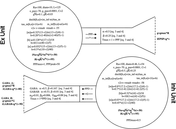
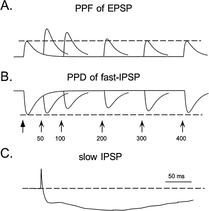
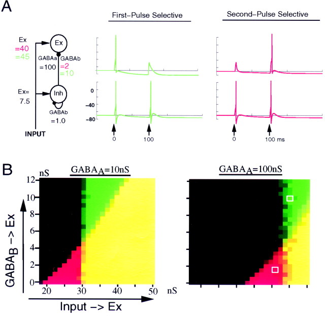
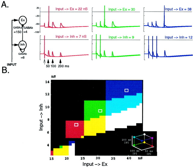
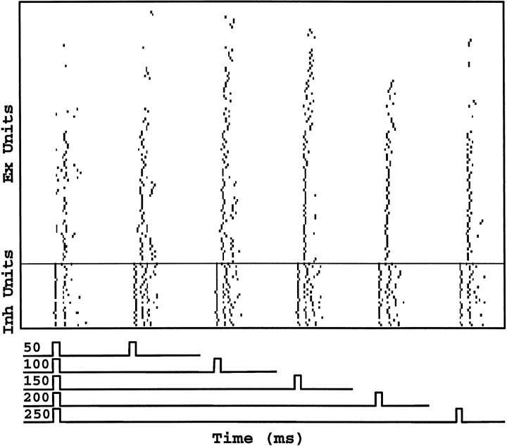
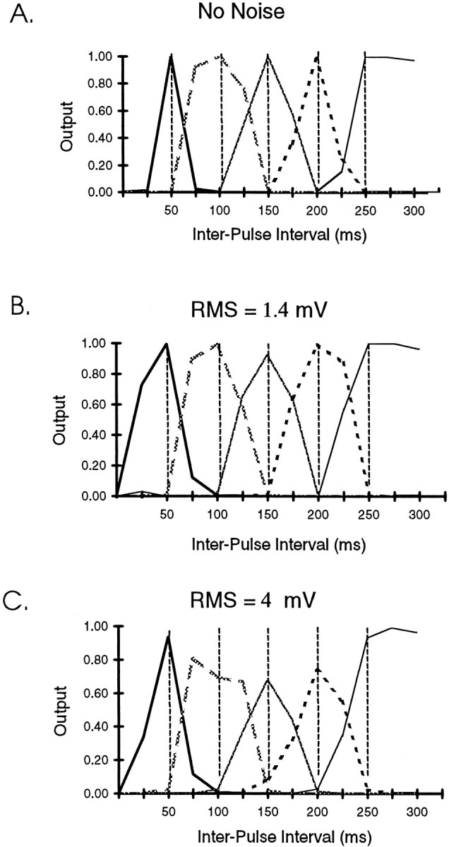
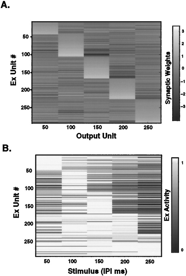
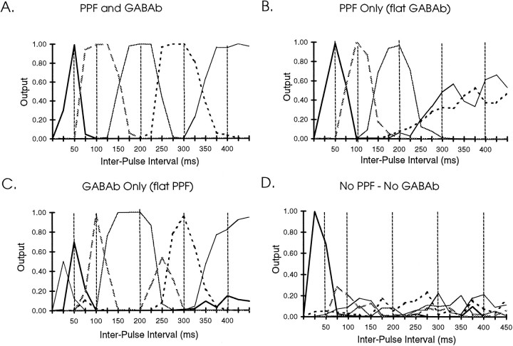
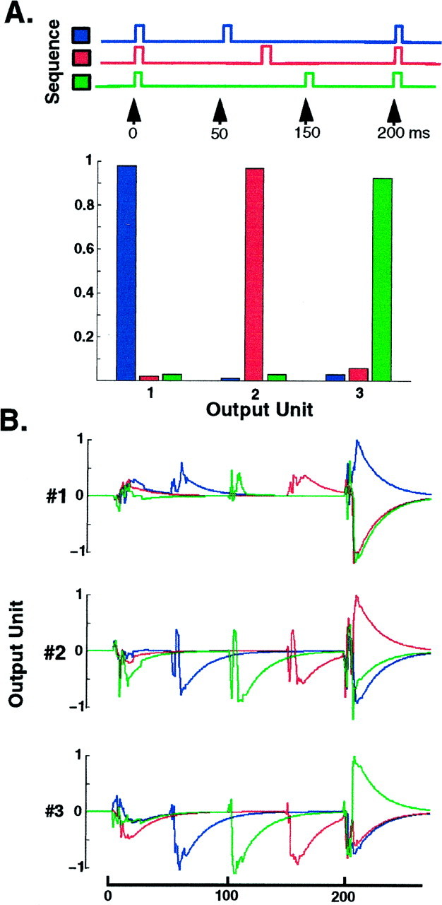
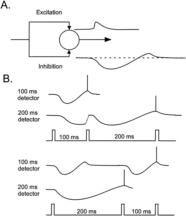
In the current paper it is proposed that short-term plasticity and dynamic changes in the balance of excitatory-inhibitory interactions may underlie the decoding of temporal information, that is, the generation of temporally selective neurons. Our initial approach was to simulate excitatory-inhibitory disynaptic circuits. Such circuits were composed of a single excitatory and inhibitory neuron and incorporated short-term plasticity of EPSPs and IPSPs and slow IPSPs. We first showed that it is possible to tune cells to respond selectively to different intervals by changing the synaptic weights of different synapses in parallel. In other words, temporal tuning can rely on long-term changes in synaptic strength and does not require changes in the time constants of the temporal properties. When the units studied in disynaptic circuits were incorporated into a larger single-layer network, the units exhibited a broad range of temporal selectivity ranging from no interval tuning to interval-selective tuning. The variability in temporal tuning relied on the variability of synaptic strengths. The network as a whole contained a robust population code for a wide range of intervals. Importantly, the same network was able to discriminate simple temporal sequences. These results argue that neural circuits are intrinsically able to process temporal information on the time scale of tens to hundreds of milliseconds and that specialized mechanisms, such as delay lines or oscillators, may not be necessary.

Fig. 1.

Equations used to simulate the Ex and Inh units. Variable names and units follow the conventions used in NEURON. The simulations consisted of separate modules for the cell somas (large circles) and synapses. The equations for the synapses are described in Materials and Methods. Parameters for PPF, PPD, and the slow IPSP were actually computed in the somatic compartment and then passed to the synaptic modules (because short-term plasticity of all the synapses of a given unit will have the same values). The arrows between both modules represent the passing of these pointer variables.

Fig. 2.

Simulated PPF of EPSPs (A), PPD of IPSPs (B), and the slow IPSP (C). EPSPs and IPSPs in the Ex unit are shown in response to paired-pulse stimulation at intervals ranging from 25 to 375 msec. Note that that some of the apparent facilitation observed in response to intervals <75 msec is attributable to temporal summation as well as actual paired-pulse facilitation.

Fig. 3.

Simulations of order selectivity.A, The panel on the left shows the disynaptic circuit and the synaptic weights. The voltage of the Ex unit (top traces) and Inh unit (bottom traces) in response to a 100 msec interval. Depending on the strength of two synapses, Input → Ex and GABA_B → Ex, the Ex unit responds selectively to the first (green) or second pulse (red). B, Parametric analysis of synapse space. Each plot varies the strength of the Input → Ex (x-axis), and GABA_B → Ex (y-axis). The strength of the GABA_A→ Ex was also varied as shown across the two subplots. Simulations were performed in the presence of noise in both units. The color scale represents the probability of firing to the first pulse and second pulse. Intense green means that given those synaptic strengths, the probability of firing to the first pulse and not to the second was 1.0. Red represents conditions in which the Ex unit responds selectively to the second pulse. Yellowrepresents nonselective responses to both pulses. Note that in each panel there is a transition along the diagonal that represents the point in which a unit changes its selectivity from the second to first pulse and that this transition points shifts to the leftacross plots.

Fig. 4.

A, Simulation of interval selectivity. The top and bottom tracesrepresent the output of the Ex and Inh unit, respectively, in response to three intervals of 50, 100, and 200 msec. The responses to each interval are overlaid. Depending on the strength of the connections onto the Ex and Inh units, the Ex unit can respond selectively to 50 (red), 100 (green), or 200 (blue) msec intervals. B, Parametric analysis of synapse space and interval selectivity displayed as an RGB plot. As color-coded in A, red represents regions of synapse space in which the Ex unit fires exclusively to the second pulse of a 50 msec IPI, but not to the 100 or 200 msec IPI, i.e., a 50 msec interval detector. Similarly, green anddark blue areas represent regions of synapse space in which the Ex units respond only to the 100 or 200 msec interval, respectively. In the same manner that a computer screen makes yellow by mixing red and green, yellow in this RGB represents conditions in which the Ex unit responded to both 50 and 100 msec intervals, but not the 200 msec interval. White areas represent regions that respond to all the intervals, but not to the first pulse. The general scheme is represented in the color cube to theright. Black areas represent regions in which the cell was not interval-selective: not firing at all or in response to the first pulse. The three unfilled white squares show the areas of synapse space of the traces inA. The other synaptic weights were GABA_A → Ex = 150 nS; GABA_B → Ex = 4 nS; GABA_B → Inh = 6 nS. The color changes in thebottom left corner reflect a more nonlinear region of synapse space corresponding to an area in which the strength of the Input → Inh synapse is still subthreshold to the first pulse but not to the second pulses.

Fig. 5.

Raster plot of a sample of Ex and Inh units in response to five different intervals. The plots in response to the five different intervals are overlaid on top of each other. Overall the number of spikes in response to each pulse was between 0 and 3. Some of the units shown were interval-selective (e.g., topmosttraces), whereas most either exhibited some preference for short intervals or were nonselective.

Fig. 6.

Interval discrimination with different levels of noise. Each plot shows the response of five outputs units, after training each output unit to one of five target intervals: 50, 100, 150, 200, and 250 msec (dashed lines). Novel stimuli representing intervals from 25 to 300 msec were used to test interval discrimination and generalization. Simulations were performed with three different levels of noise injected continuously into all the Ex and Inh units of the network. The rms of the voltage of the Ex unit wasA, 0 mV; B, 1.4 mV; and C,4 mV.

Fig. 7.

A, Synaptic weights of all the Ex units onto the five output units from the simulations shown in Figure6. Ex units are ordered according to which Output unit their strongest synapse is on, and then subordered by ascending synaptic strength.B, Interval tuning curves of the same Ex units shown inA. Interval tuning curves are made by counting the number of spikes in response to the second pulse at each interval and normalizing to the maximal response. All the units with preferred responses that were not to the first pulse are shown. Note a significant number of Ex units tuned to short intervals and broader tuning to longer intervals. The strategy of the output units was to receive strong excitatory input from the Ex units that respond selectively to the target interval and to receive strong inhibition from the units that responded to intervals shorter than the target interval.

Fig. 8.

Simulation of interval discrimination with altered time-dependent properties. In these simulations the target intervals were 50, 100, 200, 300, and 400 msec (dashed lines).A, Control results with the same parameters used in Figure 6. B, Flattened slow IPSPs and PPD. In these simulations GABA_B-dependent properties were flat 20 msec after activation, whereas PPF of EPSPs remained normal.C, Flattened PPF. D, No PPF and no GABA_B-dependent properties.

Fig. 9.

Discrimination of simple sequences.A, Average responses of the Output units trained on each stimulus to novel presentations of the three stimuli shown above.B, To understand how the output units perform sequence discrimination, we have plotted the activity of each output unit in response to each sequence. The activity plotted is simply the activity of all Ex units multiplied by the weight of the Ex → Ouput connection (and an RC time constant of 20 msec). Thus, the degree of the response to the different pulses reflects the overlap between the maximal response (last pulse of the target sequence). Distribution of the information content of all Ex units around the stimulus set.

Fig. 10.

Illustration of a labeled-line model.A, Each event produces short-lasting excitation and long-lasting inhibition followed by rebound excitation. Neither the excitation nor rebound from inhibition is capable of eliciting a suprathreshold response. If excitation from a second event coincides with rebound from the first event, threshold is reached. By adjusting the duration of inhibition (or equivalently the strength) it is possible to have labeled lines for a range of intervals.B, In the case of two stimuli composed of sequence of three pulses (each composed of a 100 and 200 msec interval), both stimuli will activate the same interval detectors, albeit in a different order. Thus, sequence discrimination will require subsequent order discrimination. One problem this type of model has with sequence discrimination is that for the appropriate labeled-line to detect the second interval, each pulse would have to “reset” the interval detector (dashed lines).

References

1. Abbott LF, Varela JA, Kamal S, Nelson SB. Synaptic depression and cortical gain control. Science. 1997;275:220–224. - PubMed
1. Adler TB, Rose GJ. Long-term temporal integration in the anuran auditory system. Nat Neurosci. 1998;1:519–523. - PubMed
1. Ahissar E, Haidarliu S, Zacksenhouse M. Decoding temporally encoded sensory input by cortical oscillations and thalamic phase comparators. Proc Natl Acad Sci USA. 1997;94:11633–11638. - PMC - PubMed
1. Beaulieu C, Kisvarday Z, Somogyi P, Cynader M, Cowey A. Quantitative distribution of GABA-immunopositive and -immunonegative neurons and synapses in the monkey striate cortex (area 17). Cereb Cortex. 1992;2:295–309. - PubMed
1. Braitenberg V. Is the cerebellar cortex a biological clock in the millisecond range? Prog Brain Res. 1967;25:334–336. - PubMed
Publication types