Spectral-temporal receptive fields of nonlinear auditory neurons obtained using natural sounds

Abstract

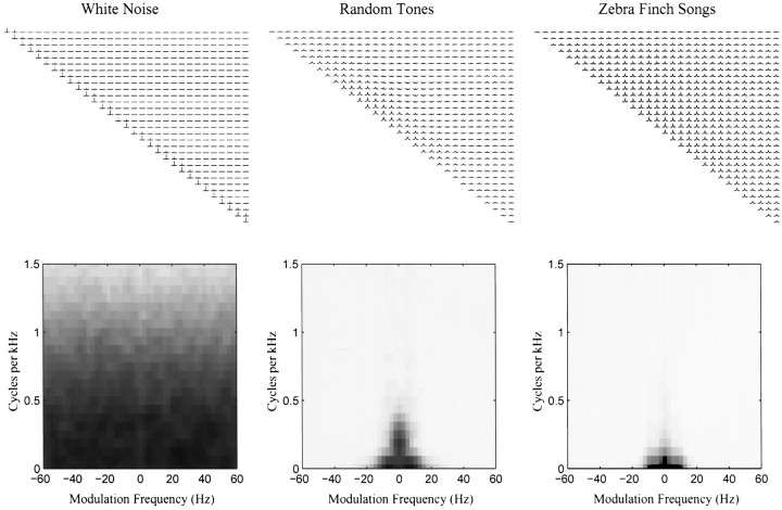
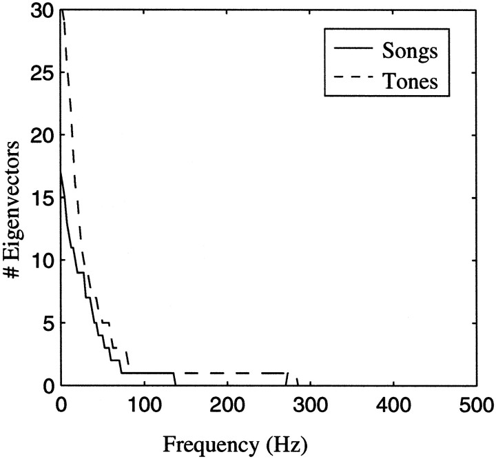
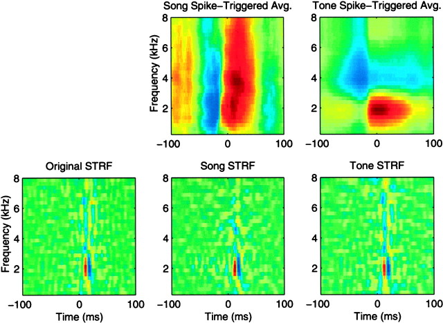
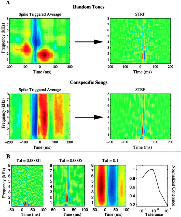
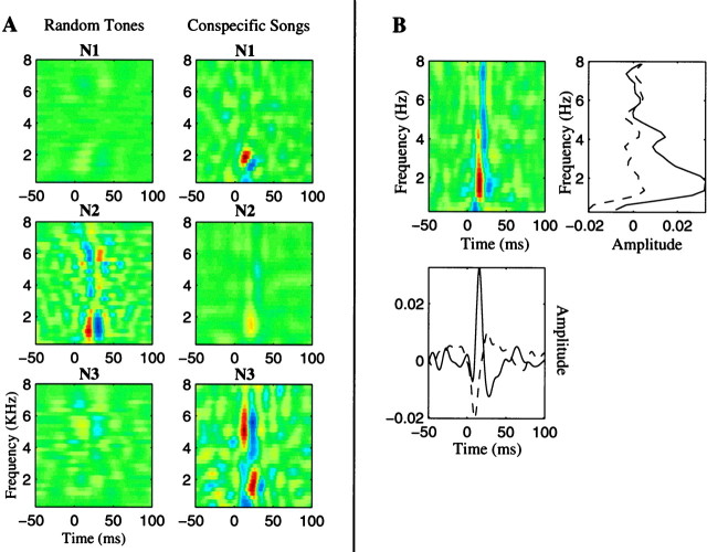
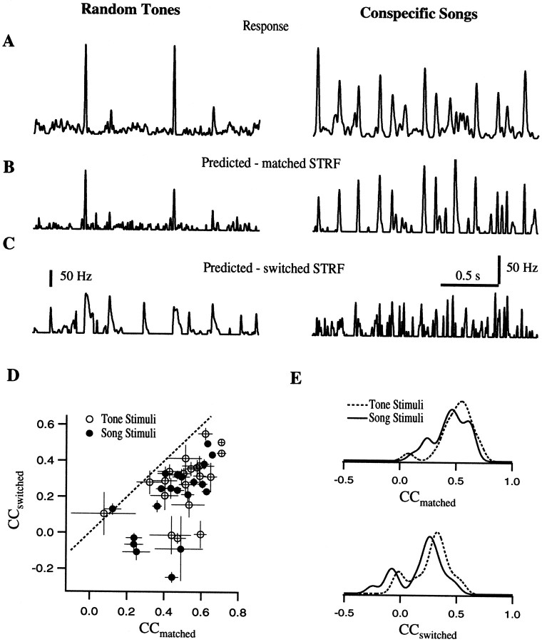
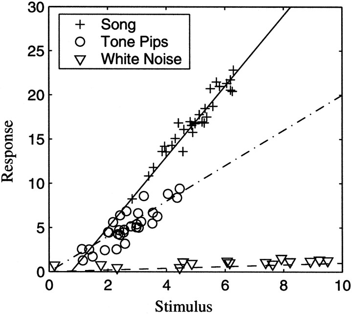
The stimulus-response function of many visual and auditory neurons has been described by a spatial-temporal receptive field (STRF), a linear model that for mathematical reasons has until recently been estimated with the reverse correlation method, using simple stimulus ensembles such as white noise. Such stimuli, however, often do not effectively activate high-level sensory neurons, which may be optimized to analyze natural sounds and images. We show that it is possible to overcome the simple-stimulus limitation and then use this approach to calculate the STRFs of avian auditory forebrain neurons from an ensemble of birdsongs. We find that in many cases the STRFs derived using natural sounds are strikingly different from the STRFs that we obtained using an ensemble of random tone pips. When we compare these two models by assessing their predictions of neural response to the actual data, we find that the STRFs obtained from natural sounds are superior. Our results show that the STRF model is an incomplete description of response properties of nonlinear auditory neurons, but that linear receptive fields are still useful models for understanding higher level sensory processing, as long as the STRFs are estimated from the responses to relevant complex stimuli.

Fig. 1.

Schematic illustrating the spectrographic decomposition and the calculation of the stimulus autocorrelation matrix. The sound is decomposed into frequency bands by a bank of Gaussian filters. The result is a set of narrowband signals with time-varying amplitude and phase. Our representation of sound is based on the time-varying amplitude envelopes. Although the time-varying phase is discarded, the relative phase across frequency bands is preserved because of the large overlap between adjoining filters. The time-varying amplitude envelope or its log is what is usually represented in a spectrogram. Our representation of sound and the spectrograms shown in this paper are based on the log of the amplitude envelopes. The stimulus autocorrelation function is then found by cross-correlating the log-amplitude envelope of a particular band with the log-amplitude envelope of all the other bands, including itself. The autocorrelation for the entire ensemble is done by averaging the correlation at each time point for all stimuli in a given ensemble. Here we show the results of two of such pairwise correlations: the correlation of band 4 (centered at 1250 Hz) with band 2 (centered at 500 Hz) and of band 4 with itself, for the song ensemble.

Fig. 2.

Power spectrum of the ensemble of 20 zebra finch songs used in this study. The curve shows the mean power density as a function of frequency. The same power density was used to generate the ensemble of tone pips.

Fig. 3.

Samples of stimuli (top panels), neuronal responses (middle panels), and mean spike rate (bottom panels) for the two stimulus ensembles: a song-like sequence of random tone pips (left column) and a zebra finch song (right column). The top panels show the spectrographic representation of the stimuli using the frequency decomposition described in Materials and Methods. Themiddle panels show 10 spike train recordings obtained in response to 10 presentations of the stimuli for a neuronal site in area L2b of one of the birds used in the experiment. The bottom panel shows the estimated spike rate obtained by smoothing the PSTH with a 6 msec time window.

Fig. 4.

Mean (A) and maximal (B) firing rates of our Field L neurons relative to background, obtained using the tone ensemble and the song ensemble.

Fig. 5.

Stimulus autocorrelation matrices (top panels) and two-dimensional power spectra (bottom panels) for a white noise ensemble and the random tone-pip and song ensembles used in this paper. The diagonal corresponds to the autocorrelation of the log of amplitude envelope of each frequency band with itself. The off diagonal terms correspond to the cross-correlation between the log of amplitude envelopes across frequency bands. The bands are ordered in increasing frequency from left toright and top to bottom. The top left corner corresponds to the autocorrelation of the amplitude envelope in the 250 Hz band. Only the top right side of the matrix is shown because it is symmetric along the diagonal (with the time axis inverted for the bottom left entries). The time window of each autocorrelation function is from −200 to +200 msec as shown in Figure 1. The ideal white noise signal would have null functions in the off-diagonal terms and delta functions in the diagonal terms. The white noise signal approaches this ideal. The random tone pip ensemble is also closer to white noise than the song ensemble but still has the spectral and temporal structure that is a result of our design (see Materials and Methods and Results). The bottom panels show the two-dimensional power spectra of the stimulus ensemble. These two-dimensional power spectra are obtained by taking the square of the two-dimensional Fourier transform of the stimulus in their spectrographic representation. The two-dimensional power spectra illustrate the temporal and spectral correlations of the stimulus in the Fourier domain. The x -axis shows the frequency of temporal modulations, and the y -axis the frequency of the spectral modulations found in spectrograms of the different sounds. The two-dimensional power spectra are symmetric around the origin and therefore only the top quadrants are shown. The two-dimensional power spectra can be obtained directly from the autocorrelation matrix of the stimulus (top row), although the reverse is only true if the correlations along the spatial (spectral) dimension are stationary.

Fig. 6.

The nature of the second-order structure in the stimulus ensembles can be assessed by estimating the number of independent dimensions (or eigenvectors) of the autocorrelation matrix as a function of the frequency of amplitude modulation, w. The random-tone pip and the song ensemble have most of their second-order structure in the low range of amplitude modulations (see Results for details).

Fig. 7.

Validation of the STRF calculation and illustration of the normalization procedure. The “Original STRF” shown in the bottom left panel of the figure was used to generate artificial neural response data for the song ensemble and tone ensemble. The model neuron was linear and had Poisson firing statistics with a similar average firing rate to the actual neurons in our data set. These artificial data were then used to obtain estimates of the STRF with our methodology. The top row shows the spike-triggered average spectrograms that are obtained from these artificial data by averaging the stimulus spectrogram around each spike in a 400 msec window. These spike-triggered average spectrograms are only equal to the STRF of the neuron if a white noise stimulus (in the time/frequency representation of choice) is used. When correlations are present in the stimulus, either in the time dimension or across the frequency bands of the spectrogram, the spike-triggered average needs to be normalized. This normalization involves a deconvolution in time and decorrelation in frequency. The STRFs obtained from the spike-triggered averages by the normalization procedure are shown on the bottom right panels. As expected, a similar STRF estimate is obtained for both ensembles and these estimates are very close to the Original STRF that was used to generate the data.

Fig. 8.

STRF calculation for a real neuron. The figure illustrates the STRF calculation explained in Results and in Figure 7 for the neuronal site of Figure 3. The calculation is based on all the responses that were obtained for the song ensemble and tone ensemble (10 trials for each of the 21 songs and 20 random tone sequences). As shown in A, for this particular neuron, the STRFs obtained from both ensembles are similar in that they exhibit similar areas of excitation. On the other hand, the spike-triggered average spectrograms were remarkably dissimilar. Most of the differences in the spike-triggered average were therefore attributable only to the statistical properties of the stimulus and not to the stimulus–response properties of this neuronal site. B shows examples of three song-based STRFs for this same neuron obtained with different noise tolerance levels, as explained in Materials and Methods. The time axis (x -axis) has been expanded from A. The normalized coherence between predicted response and actual response as a function of the tolerance level is plotted in the rightmost panel. The best predictions were obtained with a tolerance value of 0.0005.

Fig. 9.

STRFs derived using the random tone pip and song ensemble for three neuronal sites (N1–N3) with complex stimulus response properties (A) and decomposition of an STRF onto its spectral axis and temporal axis (B). In A, each row corresponds to the two STRFs that were obtained for a particular site. The left column corresponds to the STRF calculated from the random tone pip ensemble, and the right column corresponds to the STRF calculated from the song ensemble. These three examples were chosen to illustrate cases in which the STRF obtained from the random tone pip ensemble was different from the one obtained from the song ensemble. These particular sites were in L1 (N1 and N3) and L3 (N2). The STRFs differ both in amplitude and in shape. The top neuronal site can be described as being sensitive to a moving spectral edge. Similar STRFs have been found in some cortical neurons (deCharms et al., 1998). The bottom neuronal site is sensitive to a temporal combination of a low-frequency sound followed by a high-frequency sound. Both of these complex spectral-temporal responses became evident only when the song ensemble was used. In B, the STRF of the neuron of Figure 8 is projected onto its spectral axis (top right) and temporal axis (bottom left). Such analyses can be used to extract the spectral and amplitude modulation tuning of the neurons as explained in Results. Thesolid line is the projection corresponding to the largest excitatory point, and the dotted line is the projection corresponding to the largest inhibitory point.

Fig. 10.

Comparison of the predictions obtained from the two STRFs calculated for each neuronal site. A shows the actual firing rate of a particular neuronal site in response to random tone-pip stimuli (left) and to a song (right). B shows the firing rate predicted using the STRF calculated with the corresponding stimulus ensemble. C shows the predicted response calculated after switching the STRFs. This example illustrates that the STRFs obtained from the different ensembles can give radically different results. D, Scatter plot of the correlation coefficients (CC) between the predicted and the estimated firing rates, for switched STRFs versus matched STRFs. For each neuronal site, the CCs are calculated for the songs and tone pips. The solid dots show the CCs for the prediction to song stimuli, obtained either with song-STRFs (CC matched on the x -axis) or with the tone STRFs (CC switched on the y -axis). The open dots show the predictions for tone stimuli with the matched and switched filters. If the STRFs generated with the two different stimulus ensembles were identical, the points would lie on the x = y line shown in dots. Most points are below the line, although some are close to the line and some are closer to 0, showing the range of differences. E, The data in D are replotted by projecting all the points onto the x -axis (top plot) and onto y -axis (bottom plot), thus showing the individual distributions of CC-matched and CC-switched for the predictions to song and tone-pip stimuli. The distributions are obtained by convolving the raw data with a smoothing kernel of 0.05. The distribution of CC-matched for the two types of stimuli are not significantly different, but the CC-switched for the response to songs predicted using the tone STRFs are significantly smaller than the CC-switched for tone pips. In addition, all the CC-switched are smaller than or equal to the CC-matched.

Fig. 11.

For illustrative purposes, we show the distribution of stimulus response points for a hypothetical nonlinear neuron that exhibits the properties of the neurons in our data set. The multidimensional space (31 frequency bands × 400 points in time or 1600 dimensions in our case) used to represent the stimulus is collapsed onto the one-dimensional x -axis, and neural response is shown on the y -axis. White noise stimuli sample the entire space, whereas tone pips and songs only sample a region of that space. The hypothetical neuron has poor responses to white noise but significant responses to tone pips and songs, with songs being the preferred stimuli. A linear fit for each stimulus subset shows that relatively good stimulus–response predictions can be found, although the fit obtained from one ensemble is not a good model for the stimulus–response function found in a different ensemble. In particular, the fit to the white noise data is a very poor predictor. The fit to the song ensemble is better at predicting the response to tones than vice versa. The data in our ensemble exhibit similar patterns (albeit with on average much smaller correlations) in multidimensional space where the line is replaced by a hyperplane. An STRF is the set of coefficients that define such a hyperplane.

References

1. Aertsen AM, Johannesma PI. The spectro-temporal receptive field. A functional characteristic of auditory neurons. Biol Cybern. 1981a;42:133–143. - PubMed
1. Aertsen AM, Johannesma PI. A comparison of the spectro-temporal sensitivity of auditory neurons to tonal and natural stimuli. Biol Cybern. 1981b;42:145–156. - PubMed
1. Aertsen AM, Olders JH, Johannesma PI. Spectro-temporal receptive fields of auditory neurons in the grassfrog. III. Analysis of the stimulus-event relation for natural stimuli. Biol Cybern. 1981;39:195–209. - PubMed
1. Boer ED, Kuyper P. Triggered correlation. IEEE Trans Biomed Eng. 1968;15:169–179. - PubMed
1. Cai D, DeAngelis GC, Freeman RD. Spatiotemporal receptive field organization in the lateral geniculate nucleus of cats and kittens. J Neurophysiol. 1997;78:1045–1061. - PubMed
Publication types
LinkOut - more resources