QTL fine mapping by measuring and testing for Hardy-Weinberg and linkage disequilibrium at a series of linked marker loci in extreme samples of populations

Abstract

It has recently been demonstrated that fine-scale mapping of a susceptibility locus for a complex disease can be accomplished on the basis of deviations from Hardy-Weinberg (HW) equilibrium at closely linked marker loci among affected individuals. We extend this theory to fine-scale localization of a quantitative-trait locus (QTL) from extreme individuals in populations, by means of HW and linkage-disequilibrium (LD) analyses. QTL mapping and/or linkage analyses can establish a large genomic region ( approximately 30 cM) that contains a QTL. The QTL can be fine mapped by examination of the degree of deviation from HW and LD at a series of closely linked marker loci. The tests can be performed for samples of individuals belonging to either high or low percentiles of the phenotype distribution or for combined samples of these extreme individuals. The statistical properties (the power and the size) of the tests of this fine-mapping approach are investigated and are compared extensively, under various genetic models and parameters for the QTL and marker loci. On the basis of the results, a two-stage procedure that uses extreme samples and different tests (for HW and LD) is suggested for QTL fine mapping. This two-step procedure is economic and powerful and can accurately narrow a genomic region containing a QTL from approximately 30-1 cM, a range that renders physical mapping feasible for identification of the QTL. In addition, the relationship between parameterizations of complex diseases, by means of penetrance, and those of complex quantitative traits, by means of genotypic values, is outlined. This means that many statistical genetic methods developed for searching for susceptibility loci of complex diseases can be directly adopted and/or extended to QTL mapping for quantitative traits.

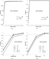
Figure 1

Illustration of the three- and five-point moving-average methods for QTL fine mapping done by use of the measure q_excess. If there are L markers genotyped, then there are L raw-data points of the point-wise disequilibrium measures. As is apparent from the figure, from these L raw-data points, there will be L-2 and L-4 data points, respectively, generated from the moving three- and five-point averages. The peaks of these three- or five-point averages indicate that the QTL is located nearby. The true location of the QTL is 0 on the X-axis. The data were obtained from one simulation, with the use of the following parameters: p=.1, p_M=.2, 2n=200, h²=.20; 100 extreme individuals were sampled from the bottom 10%, and 100 were selected from the top 10% of the phenotypic distribution, for computation of raw q_excess values (equation [11a]). The measures q_excess(1), q_excess(3), q_excess(5) indicate the data for the raw q_excess value and for the three- and five-point moving averages of q_excess, respectively.

Figure 2

Comparison of QTL fine mapping by use of different average analyses (three-, five-, and seven-point moving averages) and by use of the raw measures themselves. The q_excess was used for illustration. In simulations, p=.1, p_M=.2, 2n=200, and h²=.20, and extreme samples from the bottom 10% and the top 10% of the population were used.

Figure 3

Two-stage QTL fine mapping and comparison of the power of QTL fine mapping under the best (panels a and c) and worst (panels b and d) constellations of the QTL and the markers and with various disequilibrium measures or test statistics. The “best” and “worst” constellations refer to instances when the QTL position is the same as one marker and when the QTL is in the middle of two markers, respectively. In simulations, p=.1, p_M=.2, 2n=200, and h²=.20. The three- and five-point moving-average methods were used, respectively, in the first stage (panels a and b) and in the second stage (panels c and d) of QTL fine mapping. In the first stage, χ²₄-test statistics and the q_excess measure were used for HW and LD, with the use of 100 individuals from the bottom 10th percentile and 100 individuals from the top 10th percentile of the population. In the second stage, χ²₁, χ²₂, χ²₃, and χ²₄ statistics and D_MM , F_M , p_excess, and q_excess measures were used and compared. Since the powers of χ²₂, D_MM, and F_M are much smaller than those of the other measures or statistics, they are not presented. Panels a and b demonstrate the power of the first stage of QTL fine mapping, with genotyping of the genomic region at 1-cM intervals. Panels c and d demonstrate the power of QTL fine mapping, with genotyping of the genomic region at 0.2-cM intervals around the peaks obtained in the first stage. The genetic effect of the QTL is partial recessive for simulations in this figure and in figures 2 and 4.

Figure 4

Performance of QTL fine mapping under (a) various h², (b) various sample sizes (2n), (c) various selection criteria of the samples (5th, 10th, and 20th percentiles are respectively selected from the top and bottom distributions of the population), and (d) various degrees of LD, as measured by D⁰_A1M at the G₀ generation. χ²₃ and χ²₄ tests for HW and LD, with the use of samples from the bottom 10th percentile (100 individuals) and top 10th percentile (100 individuals) of the population, are illustrated. In simulations, unless otherwise specified, p=.1, p_M=.2, 2n=200, and h²=.20; D⁰_A1M is the maximum amount of LD simulated at the G₀ generation. After 50 generations of evolution, the expected LD is D⁵⁰_A1M=(1-c)⁵⁰D⁰_A1M.

Figure 5

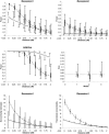
Statistical properties of the χ²₁ test (gray-shaded box) and χ²₃ test (blackened box). In simulations, p=.1 and p_M=.2, and, in the initial generation, P_A1M=.1 and D_A1M=.08. Corresponding to model 1 used by Nielsen et al. (see table 1 in Nielsen et al. [1998]), the genetic effects for the QTL (recessive 1) are: a=-50 and d=50; corresponding to model 2 (recessive 2), a=-99.62 and d=99.62; and corresponding to model 3 (additive), a=-23.45 and d=0. In these quantitative-trait models, h²=.99. Sample sizes are 2n=200. In the recessive 1, recessive 2, and additive models, the bottom 6%, 10%, and 10% of the populations were defined as “affected,” corresponding to T values of ∼50, 99, and 24, respectively. It can be easily verified, from equations (2a), (2b), and (2c), that, for the quantitative-trait model, φ₁₁, φ₁₂, and φ₁₂ are exactly the same as those in the three models used by Nielsen et al. (1998) for complex diseases. The symbols for power in the three plots represent the range of the proportions of times that the null hypothesis of no disequilibrium was rejected for the 100 simulated populations. The points joined by the connecting line are the medians, and the bottom and top edges of the boxes represent the sample 25th and 75th percentiles; the whiskers extend the range of the results. For the size plot, the symbols represent the proportion of times a true null hypothesis was rejected. The last two plots give the estimated and theoretical noncentrality parameters for the recessive 1 model.

Figure 6

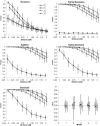
Comparison of statistical properties of different tests under various genetic models. Different symbols were used to differentiate the four tests, as is indicated on the first plot. On each plot, the data are the mean and SD at each marker (for the power plots) or for each model (the size plot), over 100 simulated populations, with each population sampled 5,000 times. Models 1–5 on the size plot correspond, respectively, to recessive (1), partial recessive (2), additive (3), partial dominant (4), and dominant (5) models. For models 1–5, the genetic parameters (a and d) are, respectively, (−2.51, 2.51), (−1.85, 0.93), (−1.18, 0), (−0.83, −0.42), and (−0.64, −0.64). For all the simulations in this figure, h²=.20, p=.10, p_M=.2, and 2n=200.

Figure 7

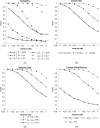
Comparison of statistical power under various parameters, with partial recessive genetic effects. In panel (1), the results for χ²₂ and χ²₄ tests are presented. In the remaining three panels (2–4), only the results for the χ²₄ test are presented. Unless otherwise specified in the panels, p=.1, p_M=.2, sample size 2n=200, and h²=.20, and extreme samples from the bottom 10% (for the χ²₂ test) or those from the bottom 10% and the top 10% of the population (the sample selection) were used for testing. Different levels of h² in panel (1), 2n in panel (2), sample selection in panel (3), and D_A1M (in the initial population at the G₀ generation) in panel (4) were indicated in the respective panels. D_A1M=P_A1M-pp_M·p_M=.5 in panel (4), and various levels of D_A1M were achieved by varying p for allele A1, which is in complete LD, in the G₀, with the marker allele M.

References

1. Allison DB (1997) Transmission-disequilibrium tests for quantitative traits. Am J Hum Genet 60:676–690 - PMC - PubMed
1. Bengtsson BO, Thomson G (1981) Measuring the strength of association between HLA antigens and diseases. Tissue Antigens 18:356–363 - PubMed
1. Bennett ST, Lucassen AM, Gough SCL, Powell EE, Undlien DE, Pritchard LE, Merriman ME, et al (1995) Susceptibility to human type 1 diabetes at IDDM2 is determined by tandem repeat variation at the insulin gene minisatellite locus. Nat Genet 9:284–292 - PubMed
1. Boehnke M (1994) Limits of resolution of genetic linkage studies: implications for the positional cloning of human disease genes. Am J Hum Genet 55:379–390 - PMC - PubMed
1. Boehnke M, Langefeld CD (1998) Genetic association mapping based on discordant sib pairs: the discordant-alleles test. Am J Hum Genet 62:950–961 - PMC - PubMed
Publication types