A thixotropic effect in contracting rabbit psoas muscle: prior movement reduces the initial tension response to stretch

Abstract

Paired ramp stretches and releases ('triangular length changes', typically 0.04 +/- 0.09L0 s-1; mean +/- s.e.m.) were imposed on permeabilised rabbit psoas fibre segments under sarcomere length control. In actively contracting fibres, the tension response to stretch was biphasic; tension rose more rapidly during the first 0. 005L0 of the imposed stretch than thereafter. Tension also dropped in a biphasic manner during shortening, and at the end of the length change was reduced below the steady state. If a second triangular length change was imposed shortly after the first, tension rose less sharply during the initial phase of lengthening, i.e. the stiffness of the muscle during the initial phase of the response was reduced in the second stretch. This is a thixotropic effect. If a third triangular length change was imposed on the muscle, the response was the same as that to the second. The time required to recover the original tension response was measured by varying the interval between triangular length changes. Recovery to steady state occurred at a rate of approximately 1 s-1. The stiffness of the muscle during the initial phase of the response scaled with the developed tension in pCa (= -log10[Ca2+]) solutions ranging from 6.3 (minimal activation) to 4.5 (saturating effect). The relative thixotropic reduction in stiffness measured using paired length changes was independent of the pCa of the activating solution. The thixotropic behaviour of contracting skeletal muscle can be explained by a cross-bridge model of muscle contraction in which the number of attached cross-bridges is temporarily reduced following an imposed movement.

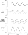
Figure 1. Mechanical response to three triangular length changes

pCa 6.0 (steady-state tension 0.38 of maximum in pCa 4.5). Length change 0.04L₀, velocity ± 0.09L₀ s⁻¹. Triangular length changes separated by 0.1 s. Dotted lines indicate steady-state tension and the initial sarcomere and segment lengths.

Figure 2. Stress-sarcomere length loop during three cycles of stretch and release

pCa 6.0 (steady-state tension 0.42 of maximum in pCa 4.5). Length change 0.04L₀, velocity ± 0.09L₀ s⁻¹. Three triangular length changes separated by 0.1 s.

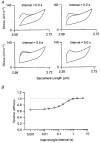
Figure 3. Time course of thixotropy

A, plots for two triangular length changes separated by a variable interval. pCa 6.1. Length change 0.04L₀, velocity ± 0.11L₀ s⁻¹. B, time course of the thixotropic effect. pCa 5.6 (steady-state tension 0.94 of maximum in pCa 4.5). Length change 0.04L₀, velocity ± 0.12L₀ s⁻¹. Muscle stiffness was calculated from the gradient of regression lines fitted to X–Y plots of tension against sarcomere length for the first 30 ms of each lengthening response. Symbols show the means ±s.e.m. (n = 3 or 4 measurements, error bars not shown where they are smaller than the symbol) of the second stretch stiffness divided by the corresponding first stretch value for each inter-triangle interval. The continuous line is a best fit of the form a – bexp(-kΔt), where a = 0.99, b = 0.43, k= 1.2 s⁻¹, and Δt is the inter-triangle interval. The dotted line indicates a relative stiffness of 1.0, i.e. the relative stiffness if the tension responses were identical.

Figure 4. Ca²⁺ dependence of mechanical responses

A, plots for a fibre segment activated in different pCa solutions. Length change 0.04L₀, velocity ± 0.09L₀ s⁻¹. Three triangular length changes separated by 0.1 s. B, the relationship between the initial stiffness and steady-state tension. Fibre segments were activated in a range of different pCa solutions and subjected to three triangular length changes (0.04L₀, velocity ± 0.05 to 0.09L₀ s⁻¹ in different preparations) once tension had reached steady state. The initial stiffness of the muscle during each lengthening phase was calculated as in Fig. 3 and expressed as a Young's modulus. Steady-state tension was normalised to the cross-sectional area of the preparation and calculated as the difference between the tension prevailing at the commencement of the first triangular length change and that measured immediately after a rapid shortening (0.2L₀) imposed once the triangular length changes were complete. Different shapes of symbols show the relationship between the first stretch stiffness and steady-state tension in five different preparations. Open symbols correspond to activating solutions with pCa values in the range 6.3 to 4.5. Closed symbols show the stiffness-stress relationship for each segment in pCa 9.0. Inset shows a linear regression line fitted to the data points with stress values below 30 kN m⁻². No systematic difference between the stiffness-stress relationship for contracting (pCa <= 6.3) and relaxed (pCa = 9.0) muscle segments is apparent. C, repeated stretches. The initial muscle stiffness for each of the three stretches and steady-state tension were expressed relative to their respective maximum values in pCa 4.5 solution (saturating effect). Symbols show the means ±s.e.m. values of tension (○), first stretch stiffness (□), second stretch stiffness (▵) and third stretch stiffness (•) in each pCa solution. Lines show best fits for each data set of the form y=[Ca²⁺]^n_H/([Ca²⁺]^n_H+x₅₀^n_H), where n_H is the Hill coefficient and x₅₀ is the apparent dissociation constant. Fit parameters: tension, n_H= 2.59, x₅₀= 5.86; first stretch stiffness, n_H= 2.89, x₅₀= 5.78; second stretch stiffness, n_H= 2.95, x₅₀= 5.78; third stretch stiffness, n_H= 2.97, x₅₀= 5.80.

Figure 5. Break length for force response to stretch

A, schematic diagram illustrating the technique used to identify the break length ΔL. Muscle stress was plotted against sarcomere length for the lengthening phase of the first triangular length change. A linear regression line (thick continuous line) was then calculated for the first 30 ms of lengthening (beginning and end points marked by vertical arrows) and extrapolated to the maximum tension reached during the initial phase of the response (horizontal dashed line, positioned by eye). The break length ΔL was calculated from the imposed length change at this intercept and expressed in units of nanometres of extension per half-sarcomere. In this example ΔL was 6.24 nm (half-sarcomere)⁻¹. B, break lengths at different levels of Ca²⁺ activation. Fibre segments were activated in a range of different pCa solutions and subjected to three triangular length changes (0.04L₀, velocity ± 0.05 to 0.09L₀ s⁻¹ in different preparations) once tension had reached steady state. Steady-state tension was expressed relative to the maximum value in pCa 4.5 solution (saturating effect). Different symbols show the break length-relative tension relationship for the first lengthening response in different preparations. The mean calculated break length was 6.23 ± 0.24 nm (half-sarcomere)⁻¹; 45 measurements from five different fibre segments. This corresponds to an extension of ≈0.005L₀. We were unable to develop a method which unambiguously defined the break length in the second or third length changes.

Figure 6. Simulated mechanical response to three triangular length changes

Fifteen model parameters were adjusted to optimise the fit between the simulated tension response and the experimental record (pCa 6.0, length change 0.04L₀, velocity ± 0.09L₀ s⁻¹, three triangular length changes separated by 0.1 s) shown in Fig. 2. Stress records: thick continuous line, muscle stress (i.e. cross-bridge force F_cb+ parallel component force F_p); thin line with noise, experimental record; dotted line, force due to cross-bridges in first attached (A₁) state; dashed line, force due to second attached (A₂) state (power-stroked) cross-bridges; dashed-dotted line, parallel component force F_p. Proportion of attached cross-bridges simulations: continuous line – proportion of cross-bridges attached in either state; dotted line, proportion of cross-bridges attached in A₁ state; dashed line, proportion of cross-bridges attached in A₂ state. Sarcomere length: sarcomere length during triangular length changes.

Figure 7. Simulations of the thixotropic effect

A, simulated X–Y plots for two triangular length changes separated by a variable interval. Tension responses to two triangular length changes (length change 0.04L₀, velocity ± 0.09L₀ s⁻¹) separated by 0.0, 0.2, 0.5 and 5.0 s were simulated using model parameters identical to those used in Fig. 6. B, simulated thixotropic time course. The time course of the simulated thixotropic effect was quantified using a method identical to that described in the legend of Fig. 3 except that the stiffness values were calculated from the first 10 ms of the lengthening response. The continuous line is a best fit of the form (a – bexp(-kΔt), where a = 1.00, b = 0.35, k= 3.1 s⁻¹, and Δt is the inter-triangle interval.

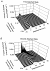
Figure 8. Redistribution of cross-bridge populations during repeated movements

A, first attached (A₁) state. B, second attached (A₂) state. These diagrams illustrate the results of simulations of repeated stretches (0.16L₀ s⁻¹ starting at t = 0 s). Each strip indicates the number of cross-bridges (vertical z-axis) attached with the corresponding elastic element length (Displacement, horizontal x-axis). The y-axis running ‘into’ the page shows the elapsed time since the commencement of the stretch. Cross-bridge distributions for two different initial conditions are shown by alternating strips. Black strips represent the simulated cross-bridge distributions during a single ramp stretch imposed at steady state from a constant length. White strips represent the simulated distributions for an identical ramp stretch imposed immediately after (inter-stretch interval = 0 s) a ‘conditioning’ triangular length change (0.04L₀, velocity ± 0.16L₀ s⁻¹). The simulated distributions for the first attached state (A₁) are very similar in each stretch because the mean life time of a cross-bridge in this state is short in comparison with the stretch velocity. In contrast, the distributions for the much longer-lived second attached state (A₂) are substantially different at the beginning of each stretch but reach the same steady-state configuration during the latter stages of the movement. Simulation parameters are identical to those used in Figs 6 and 7.

Figure 9. Theoretical model

A, overview. The model simulates the behaviour of a theoretical ‘half-sarcomere’ of unit cross-sectional area. The force per unit area in the muscle, F, is the sum of the stresses in the parallel elastic component, F_p, and the cross-bridge component, F_cb. F_p is a single-valued function of the length X of the half-sarcomere. F_cb is calculated from simulations of the cross-bridge cycling scheme. The initial length of the model is assumed to correspond to a half-sarcomere length of 1.3 μm. Thus an imposed stretch of 0.01L₀ would increase X from 0 to 13 nm. B, cross-bridge cycling scheme. Cross-bridges are assumed to act as linear elastic elements (stiffness κ_cb) and can exist in one of three distinct states: D (detached), A₁ (first attached) and A₂ (second attached). The length, x, of the elastic element (referred to as the cross-bridge displacement) defines both the force in the cross-bridge linkage and the probability of the cross-bridge undergoing a transition to a different state, i.e. the rate constants k₁, k_-1, k₂, k_-2 and k₃ are strain dependent. The transition between the A₂ and D states is assumed to correspond to the hydrolysis of one molecule of ATP and is irreversible in our simulations.

Figure 10. Rate constants

Strain dependence of the rate constants for cross-bridge transitions. A, D ⇌ A₁. Continuous line k₁(x), dashed line k_-1(x). B, A₁→A₂. C, A₂→D. The rate constants defining the probability of a cross-bridge undergoing a transition to a different state depend on the displacement x of the elastic element of the cross-bridge. The functional forms of the rate constants are given in eqns (A6) to (A10). The parameter values represented here were found by multidimensional optimisation routines and are shown in Table 1. Note the y-axis breaks in A and C which allow the strain dependence of the detachment rate constants for both negative and positive cross-bridge displacements to be illustrated in the same graph.

References

1. Bagni MA, Cecchi G, Colomo F, Garzella P. Are weakly binding bridges present in resting intact muscle fibers? Biophysical Journal. 1992;63:1412–1415. - PMC - PubMed
1. Bagni MA, Cecchi G, Colomo F, Garzella P. Absence of mechanical evidence for attached weakly binding cross-bridges in frog relaxed muscle fibres. The Journal of Physiology. 1995;482:391–400. - PMC - PubMed
1. Bartoo ML, Linke WA, Pollack GH. Basis of passive tension and stiffness in isolated rabbit myofibrils. American Journal of Physiology. 1997;273:C266–276. - PubMed
1. Brenner B. Effect of Ca2+ on cross-bridge turnover kinetics in skinned single rabbit psoas fibers: Implications for regulation of muscle contraction. Proceedings of the National Academy of Sciences of the USA. 1988;85:3265–3269. - PMC - PubMed
1. Buchthal F, Kaiser E. The rheology of the cross striated muscle fibre with particular reference to isotonic conditions. Det Kongelige Danske Videnskabernes Selskab Biologiske Meddelser, Copenhagen. 1951;21:1–307.
Publication types
LinkOut - more resources