Changes in brain cell shape create residual extracellular space volume and explain tortuosity behavior during osmotic challenge

Abstract

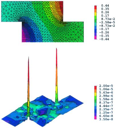
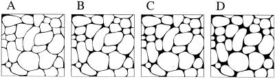
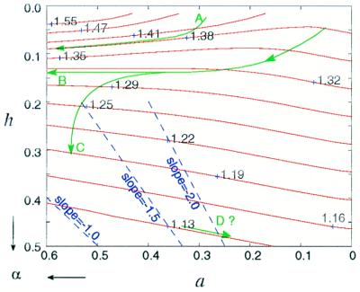
Diffusion of molecules in brain extracellular space is constrained by two macroscopic parameters, tortuosity factor lambda and volume fraction alpha. Recent studies in brain slices show that when osmolarity is reduced, lambda increases while alpha decreases. In contrast, with increased osmolarity, alpha increases, but lambda attains a plateau. Using homogenization theory and a variety of lattice models, we found that the plateau behavior of lambda can be explained if the shape of brain cells changes nonuniformly during the shrinking or swelling induced by osmotic challenge. The nonuniform cellular shrinkage creates residual extracellular space that temporarily traps diffusing molecules, thus impeding the macroscopic diffusion. The paper also discusses the definition of tortuosity and its independence of the measurement frame of reference.

Figure 1

Schematic diagrams of the two-dimensional lattice arrangements in different situations. Impermeable cell obstacles are represented by the depicted gray-colored cells arranged in a lattice structure. The distance 2h represents the intercleft width, and the radius a represents the small curvature of the cell membrane in deformed regions. The ECS domains were highlighted in light gray, with the rectangular dimension Γ_x × Γ_y defined as: Γ_x = Γ_y = 1 for lattice (a); Γ_x = Γ_y = for lattice (b); Γ_x = 2, Γ_y = 1 for lattice (c); Γ_x = , Γ_y = 1 for lattice (d); and Γ_x = , Γ_y = 3 for lattice (e).

Figure 2

Numerical solutions (Upper) of Eq. 2 by pltmg (25) and the ℋ₁ error estimates (Lower) for the staggered lattice arrangement (c) with a = 0, h = 0.5, and ê aligned with the x axis. The ℋ₁ norm, defined as ∥e_h∥_ℋ1 ≡ [∫_Ωe_h²dΩ + ∫_Ω(∇e_h)²dΩ]^1/2 (25), estimates the sum of the magnitudes of the error itself and the gradient of the error. For visual clarity, only 1,000 vertices were shown.

Figure 3

Distributions of λ vs. a and h for each lattice arrangement depicted in Fig. 1, except the diamond formation (b) displayed in the form of the difference λ^(a) − λ^(b). Superscripts in λ denote the lattice arrangement, and subscripts (x or y) denote the direction of the macroscopic diffusion ê. If λ_x = λ_y, the subscripts x, y are omitted. Judging from the smallness of λ^(a) − λ^(b), we concluded that the difference between λ^(a) and λ^(b) arose purely from numerical errors, not because of intrinsic differences in lattice structure or orientations of ê.

Figure 4

Configurations of the more realistic brain extracellular space, computer generated to mimic the two-dimensional section of neuropil ultrastructure commonly seen in electron microscopy. The fractions of the void area, α, were calculated to be 0.13 in A, 0.16 in B, 0.18 in C, and 0.22 in D.

Figure 5

Triangulation of the ECS domain (12 × 12) by pltmg for case D (α = 0.22) in Fig. 4 with 1,000 vertices. Subset shows the corresponding numerical solution for ê aligned in the x axis.

Figure 6

Contour distribution of the λ in lattice arrangement (a). Along each contour line (red), the value of λ, labeled by the nearby numbers, remains constant. Arrows at the lower-left corner indicate the directions of increasing α, which coincide with the directions of increasing a and h. Thick green curves denote possible paths of cell-shape changes during osmotic challenge. Dashed blue lines indicate the paths that preserve the shape perspective during shrinking with a constant slope defined as (1 − h)/a.

Figure 7

Comparison of theoretical and experimental λ vs. α. The theoretical line represents trace B in Fig. 6 derived from calculations by using arrangement a in Fig. 1. Experimental data are taken from ref. and J. Kume-Kick, T. Mazel, I. Vor̆ís̆ek, L. Tao, S. Hrabĕtová, & C. N. (unpublished work). Arrows on curves indicate appropriate ordinates and abscissa.

References

1. Allbritton N L, Meyer T, Stryer L. Science. 1992;258:1812–1815. - PubMed
1. Francis K, Palsson B O. Proc Natl Acad Sci USA. 1997;94:12258–12262. - PMC - PubMed
1. Agnati L F, Zoli M, Stromberg I, Fuxe K. Neuroscience. 1995;69:711–726. - PubMed
1. Agnati L F, Fuxe K, Nicholson C, Syková E. Volume Transmission Revisited. Amsterdam: Elsevier; 2000.
1. Morrison P F, Laske D W, Bobo H, Oldfield E H, Dedrick R L. Am J Physiol. 1994;266:R292–R305. - PubMed
Publication types
LinkOut - more resources