Coding of border ownership in monkey visual cortex

Abstract

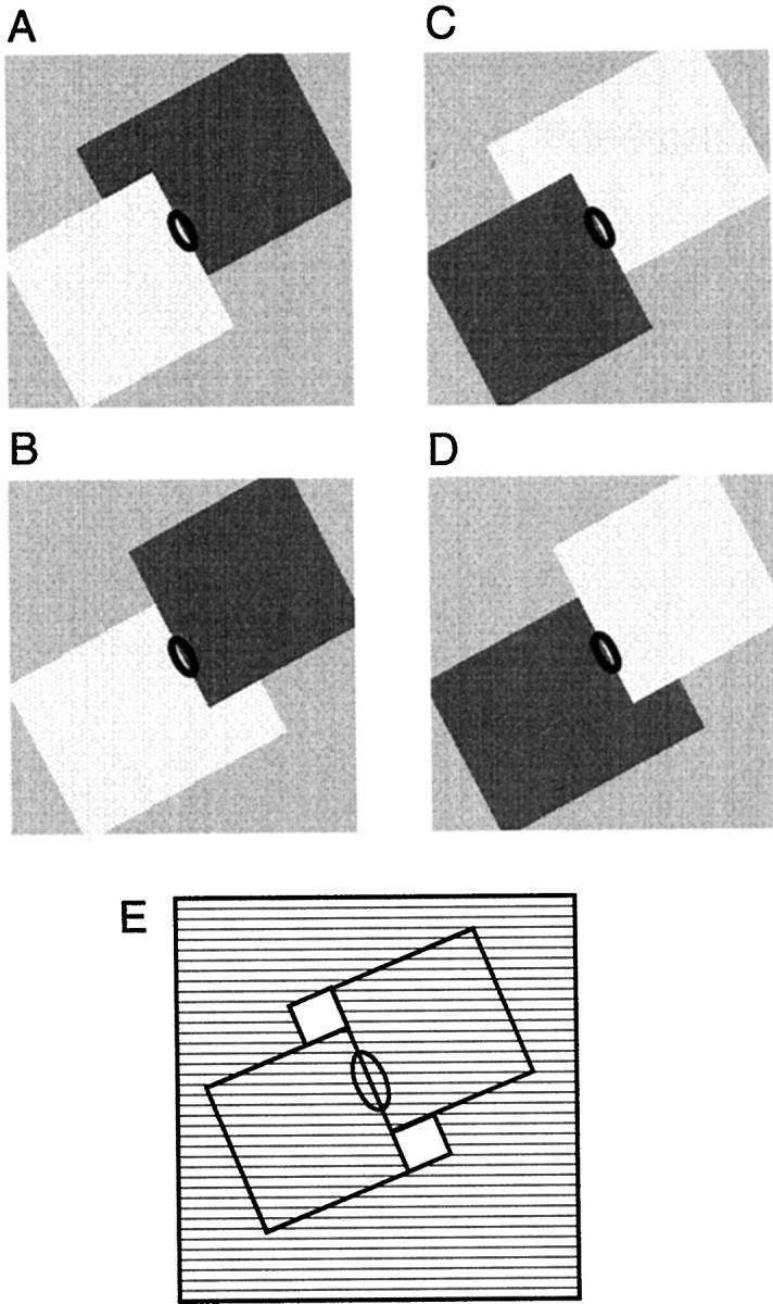
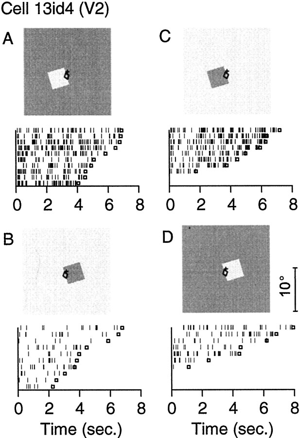
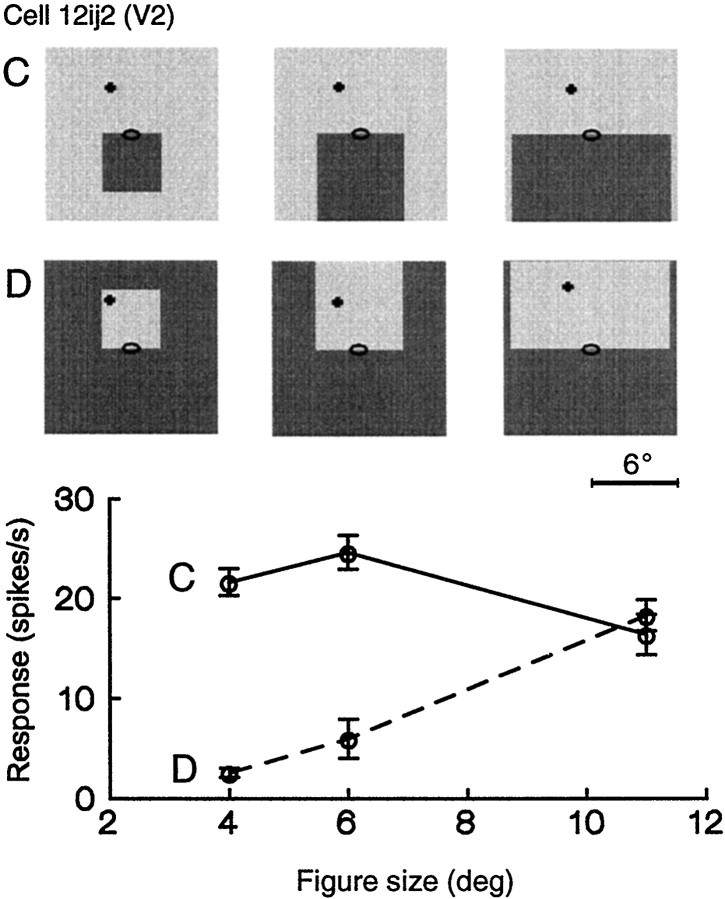
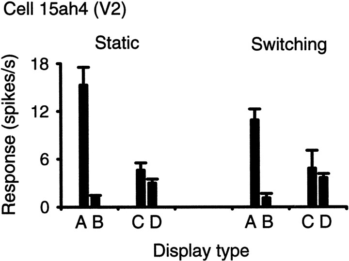
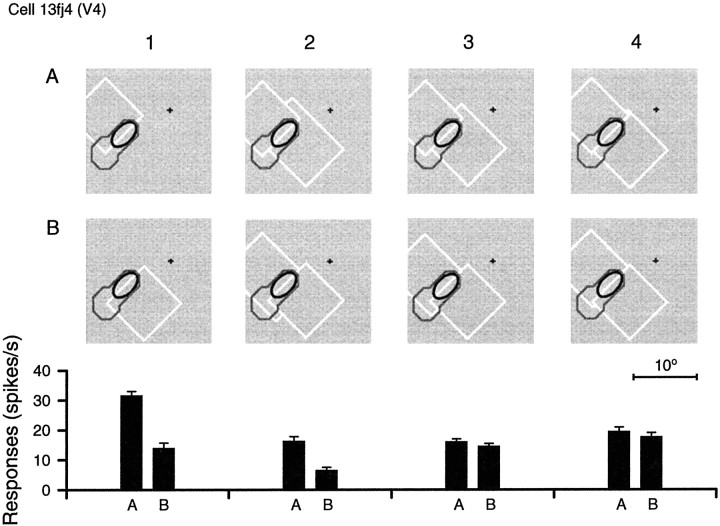
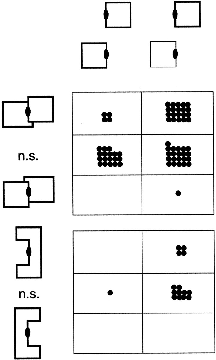
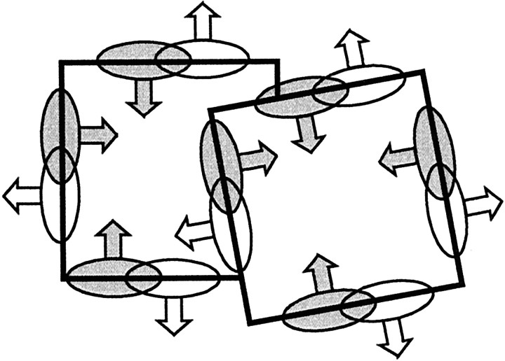
Areas V1 and V2 of the visual cortex have traditionally been conceived as stages of local feature representations. We investigated whether neural responses carry information about how local features belong to objects. Single-cell activity was recorded in areas V1, V2, and V4 of awake behaving monkeys. Displays were used in which the same local feature (contrast edge or line) could be presented as part of different figures. For example, the same light-dark edge could be the left side of a dark square or the right side of a light square. Each display was also presented with reversed contrast. We found significant modulation of responses as a function of the side of the figure in >50% of neurons of V2 and V4 and in 18% of neurons of the top layers of V1. Thus, besides the local contrast border information, neurons were found to encode the side to which the border belongs ("border ownership coding"). A majority of these neurons coded border ownership and the local polarity of luminance-chromaticity contrast. The others were insensitive to contrast polarity. Another 20% of the neurons of V2 and V4, and 48% of top layer V1, coded local contrast polarity, but not border ownership. The border ownership-related response differences emerged soon (<25 msec) after the response onset. In V2 and V4, the differences were found to be nearly independent of figure size up to the limit set by the size of our display (21 degrees ). Displays that differed only far outside the conventional receptive field could produce markedly different responses. When tested with more complex displays in which figure-ground cues were varied, some neurons produced invariant border ownership signals, others failed to signal border ownership for some of the displays, but neurons that reversed signals were rare. The influence of visual stimulation far from the receptive field center indicates mechanisms of global context integration. The short latencies and incomplete cue invariance suggest that the border-ownership effect is generated within the visual cortex rather than projected down from higher levels.

Fig. 1.

Perception of border ownership. A, Rubin's vase (Rubin, 1915). This well known ambiguous figure demonstrates the tendency of the visual system to interpret contrast borders as occluding contours and to assign them to one of the adjacent regions. In this example, figure-ground cues have been carefully balanced, but the black and white regions are generally not perceived as adjacent; instead, perception switches back and forth, and the borders belong either to the vase or to the faces. B, Isolated regions of contrast are generally perceived as “figures”, that is, objects seen against a background. C, This display is generally perceived as two overlapping rectangles rather than a rectangle adjacent to an L-shaped object.

Fig. 2.

The standard test for determining the effect of border ownership on edge responses. In A andB, identical contrast edges are presented in the receptive field (ellipses), but in A, the edge is the right side of a dark square, in B, it is the left side of a light square. The relation is analogous betweenC and D, with reversed contrasts.E, The hatched region indicates the neighborhood of the receptive field in which displays Aand B (or C and D) are identical. The preferred color of the cell (including black,white, and gray) and a light gray were used as the colors in these displays.

Fig. 3.

Overlapping figure test. In each of these displays two regions of approximately the same area are presented on either side of the receptive field (ellipses). As in Figure 2, the contrast edges in the receptive field were identical inA and B and in C andD but belonged perceptually to different figures. InE, the hatched area indicates the region of identical stimulation.

Fig. 4.

Example of border-ownership coding in a cell of area V2. The stimuli are shown at the top, and event plots of the corresponding responses are shown at thebottom. The ellipses indicate the location and orientation of the receptive field, and thecrosses show the position of the fixation target. In the event plots, small vertical lines represent the times of action potentials, relative to the moment of lever pulling (which generally indicated the beginning of fixation). Small squares indicate the times of target flip (end of fixation). Each row represents a trial. Several repetitions are shown for each condition, sorted according to the length of the fixation period. A, B, The cell responded better to the edge of a green square on the left side than to the edge of gray square on theright side of the receptive field, although both stimuli were locally identical (green depicted here aslight gray). C, D, When the colors were reversed, the cell again responded better to an edge that belonged to a square on the left than a square on theright. Square size, 4°; length of minimum response field, 0.4°; location in visual field (0.0°, −1.7°).

Fig. 5.

Size invariance of border-ownership coding. The same V2 cell as in Figure 4. Rows A and Bshow the stimuli, with pairs of locally identical stimuli juxtaposed. Conventions as in Figure 4. Bar graphs below show mean firing rates and SEs of the corresponding responses. Square sizes: 1 and 2, 4°; 3 and 4, 10°; 5 and 6, 15°. For each size, and for either contrast polarity, the responses were stronger when the square was located on the left side of the receptive field.

Fig. 6.

Selectivity for local contrast polarity. Cell of layer 2/3 of V1. The cell responded more strongly to light–dark edges (A, B) than to dark–light edges (C, D) irrespective of the position of the figure. The colors wereyellow (depicted as light gray) andgray. Location of receptive field (−1.1°, −1.1°).

Fig. 7.

Example of simultaneous coding of border-ownership and edge-contrast polarity. This cell of area V2 was color-selective with a preference for dark, reddish colors (see Fig. 8).Brown and gray were used for the test. Conventions are the same as for Figure 4. The cell responded to thetop edge of a brown square(C), but hardly at all to thebottom edge of a gray square (D), although in both cases the same gray–brown color boundary was presented in the receptive field. The cell did not respond at all to edges of the reversed contrast (A, B). Square size, 4°; length of minimum response field, 1.4°; location in visual field (1.4°, −3.0°).

Fig. 8.

The color selectivity of the cell of Figure 7. Bars of 15 colors (Table 1) were flashed in the receptive field for 500 msec with intervals of 500 msec. The graph represents mean firing rates with SEs. Activity during the On phases is plotted upward, and activity during the Off phases is plotted downward. It can be seen that the cell responded to reddish hues better than to greenish hues, with a preference for the darker representative of each hue (brown > red, beige >yellow, black > white, etc.). Whereas, in most cells, the demonstration of border-ownership coding did not require chromatic stimuli, cells with striking chromatic selectivity were also common.

Fig. 9.

Size invariance of border-ownership coding in the color-selective cell of Figures 7 and 8. Side of ownership produced response differences for 4 and 6° squares, but not for squares of 11° size. Human observers also find the distinction of figure and ground weak for the largest size. Colors were brown andgray, here depicted as dark andlight gray.

Fig. 10.

Eye movements during fixation. Recordings from monkey M16 during the standard test displays with 4° squares.a–c, Means and SDs of horizontal and vertical positions of gaze, grouped according to display type (Fig. 2,A–D). Each plot represents ∼320 trials with stimulus orientations of 135° (a), 45° (b), and 135° (c) recorded in succession. If the side of the square had influenced gaze position systematically, means A and Cwould appear displaced relative to means B andD in the direction perpendicular to stimulus orientation. No systematic displacements were apparent.d, Histogram shows the distribution of the effects of figure position on eye movements perpendicular to stimulus orientation, as determined by ANOVA, in 101 blocks of 40 trials each. Positive values designate eye movements that would have moved the receptive field toward the center of the figure. Binwidth, 3 arc min. The eye movements were small and not systematically related to the side of the figure.

Fig. 11.

Position invariance of border ownership coding in a cell of V2. The top left edge of a light square (A), and the bottom right edge of a dark square(B), were centered on the receptive field, and position of the squares was then varied. Mean firing rates and SEs are plotted as a function of edge location relative to receptive field center. Open circles represent responses to edge oflight square (A), andfilled circles represent responses to edge ofdark square (B). In either case, the maximum response was obtained when the edge was centered on the receptive field, but the responses were stronger for Athan for B at any position. SA, Level of spontaneous activity. Ellipse, Minimum response field.Cross, Fixation target. Line indicates range of variation of edge position, positive toward bottom right. Colors were aqua and gray; size of square, 4°; receptive field location (0.4°, −1.7°).

Fig. 12.

Position invariance of border ownership coding in a cell of V4. The cell responded to the top edge of thelight figure (A), but not thebottom edge of the dark figure (B) at any position. SA, Spontaneous activity. Straight line indicates range of variation of edge position, positive downward. Ellipsedelineates the most sensitive region of the receptive field (approximate contour of half-maximal response), the gray line the more uncertain total extent (note that the short axis of the ellipse corresponds to the preferred orientation of the cell). Colors, yellow and light gray; width of figure, 10°; receptive field location (4.6°, −4.9°).

Fig. 13.

Comparison of conventional receptive field size and extent of image context integration. Responses of a cell of V2.A, Firing rate as a function of the position of a 0.2° wide, 1° long static white bar on graybackground. The bar was presented at the preferred orientation of the cell, and position was varied along that orientation (right) and along the orthogonal axis (left). Insets show the bar at positions +1 and −1°, corresponding to the end points of the plotted curves.Ellipse indicates the region outside which the bars did not evoke a response (“minimum response field”; note that the preferred orientation is that of the short axis of the ellipse).Dashed lines indicate level of spontaneous activity.B, Responses to an edge of a static square of 8° size at various positions along the preferred orientation. Stimulus displays are illustrated for three data points (arrows). The responses were approximately constant as long as the edge remained inside the minimum response field and dropped to zero when the edge left the field. C, Test for border ownership.Open bars, Responses to white squares;filled bars, responses to gray squares.Despite its small receptive field, the cell differentiated displays that were identical in an 8 × 16° region around the receptive field. Note different scales of stimulus insets in Aversus B and C. Colors,white and light gray; receptive field location (0.2°, −1.7°).

Fig. 14.

Static and switching displays produced similar results. Responses from a cell of V2 that was selective for border ownership and contrast polarity. The labels refer to the displays of Figure 2. Colors red and gray were used.

Fig. 15.

The distributions of the magnitude of the border-ownership effect in the three cortical areas V1, V2, and V4. Theresponse ratio is the ratio of the mean response to the nonpreferred side over the mean response to the preferred side.

Fig. 16.

The distributions of the types of contour responses found in cortical areas V1, V2, and V4. Classification based on two-factor ANOVA. Ownership, Responses modulated according to side of ownership; contrast, responses modulated according to local contrast polarity; ownership & contrast, modulation by either factor; none, no modulation. In V2 and V4, more than half of the cells showed border-ownership modulation. Note that there are fewer cells in this figure than in Figure 15 because cells tested only with outlined figures are not included here.

Fig. 17.

A decision model used to estimate the reliability of border ownership signals. The model assumes four neuronsA–D with identical receptive fields except for reversals of side preference and contrast polarity preference, as indicated by the symbols (tabs for side preference, fill pattern for contrast polarity preference). The decision was based on the responses of these four neurons combined in the form (A − B) + (C − D). Because the four model neurons have otherwise identical response properties, recording the responses of one of them to the four stimuli of Figure 2 provides the responses of all four neurons to any one stimulus. The analogous model was used for local contrast discrimination; in this case the decision was based on the signal (A −C) + (B −D). See Results for explanation of how reliability estimates were calculated.

Fig. 18.

The reliability of neural responses in signaling border-ownership and local contrast polarity. Each dotrepresents the reliability estimates for one neuron derived from 1 sec samples of activity as explained in Results (0.5 = random, 1.0 = perfectly consistent). The histograms show distributions of reliability estimates for each dimension. Cells that reliably signaled edge-contrast polarity were common in V1 (dots attop of scatter plot). Their relative frequency was similar in the extrastriate areas, as shown by histograms onright margins. Cells that signaled border ownership were rare in V1, but common in V2 and V4 (dots nearright margins). Substantial fractions of cells signaled both border ownership and polarity of contrast (dots intop right corners).

Fig. 19.

The effect of figure size on border ownership discrimination in cortical areas V1, V2, and V4. Eachpoint represents a reliability estimate based on a test with one size; points for the same cell are connected bylines. The figure size generally had little effect.

Fig. 20.

The time course of border-ownership modulation. The figure shows the average responses of all neurons with significant border-ownership modulation in the three areas. The responses of each cell were normalized to its mean firing rate during the fixation period and averaged. Zero on the time scale refers to the onset of the figure-ground display. Thick and thin lines represent responses to preferred and nonpreferred sides, averaged over both contrast polarities. A differentiation was evident shortly after the response onset for cells in all three cortical areas.

Fig. 21.

Border-ownership coding and stereoscopic edge selectivity. Responses of two cells of V2. Circlesconnected by lines show position-response curves obtained with random-dot stereograms (r.d.s.) portraying a 4° square. Disparity of square was set to optimum (7 arc min “near” for the left cell, 14 arc min “near” for right cell), and background disparity was zero. Position of square was varied orthogonally to preferred orientation. Arrows indicate positions at which edges were centered in the minimum response fields, as illustrated above. Square symbols represent responses to edges of uniform squares of two contrast polarities, as specified in legend. It can be seen that both cells responded selectively to one side of the square, and that the preferred sides were the same for contrast-defined and disparity-defined squares. Because random-dot stereograms define border ownership unequivocally, these results confirm the assumption that the side preferences for contrast-defined figures reflect border ownership coding. Location of receptive fields: left cell (2.9°, −1.6°), right cell (−3.2°, −3.1°).

Fig. 22.

Consistent border-ownership coding forsolid and outlined squares. Cell of V4. Conventions of receptive field map as in Figure 12. Colors weregray and pink (depicted aswhite). Line width, 0.2°.

Fig. 23.

Example of a V2 cell tested with single squares, C-shaped figures, and overlapping figures. The cell was color-selective with a preference for violet.1, 2, In the standard test the cell was found to be selective for border ownership and local contrast polarity, responding best to the edge of aviolet square located on the bottom left-hand side of the receptive field (A1).3, 4, With C-shaped displays, the cell responded better to B3, in which a violet C-shape was located on the bottom left, than to A3, in which the central portion was similar to A1. 5, 6,With overlapping figures, the cell responded to theviolet–gray edge better when the violetfigure appeared to be laid on top of a gray figure (A5) than when a gray figure appeared to be laid on top (B5). Location of receptive field (0.2°, −0.4°).

Fig. 24.

Example of a V4 cell tested with single squares, C-shaped figures, and overlapping figures. Ellipseindicates minimum response field. 1, 2, In the standard test, this cell showed a preference for figure location on theright (B) with both contrast polarities. The same side was preferred for C-figures (3A, 4A), but for the overlapping figures, response differences were not significant (5, 6). Colors:1–4, green (depicted here aswhite) and light gray; 5, 6, green, light gray, anddark gray. Location of receptive field center (0.5°, −5.2°).

Fig. 25.

Responses of a cell of V4 to outlined squares and outlined overlapping figure displays. For the largest overlap (1.7 × 3.3°) the response difference was consistent with the side preference for single squares, but for smaller overlaps (1.7 × 1.7° and 0.5 × 0.5°) border ownership did not make a difference. White lines on gray, line width, 0.2°. Conventions of receptive field map as in Figure 12. Location of receptive field center (−7.4°, −3.9°).

Fig. 26.

Responses of a cell of V2 (same cell as in Fig.4). This cell showed contrast-independent side preference for edges of squares (1, 2). For C-figures, no side differentiation was found (3, 4). Instead, the responses now differed according to local contrast polarity. Colorsgray and olive (depicted as dark gray) were used.

Fig. 27.

Summary of the results obtained with single squares, overlapping figures, and C-shaped figures. Eachdot represents a cell tested. The right column represents cells with significant side preference for single squares, the left column represents cells with no significant preference. This is indicated schematically at thetop, where line thickness represents response strength. The rows correspond to the side preferences in the other tests, as indicated on theleft. If a significant (p < 0.01) side preference was found for overlapping figures, or C-figures, it was consistent with the single-figure result, except for one cell in which preference was reversed for overlapping figures. However, many cells with significant side preference for single squares failed to differentiate border ownership in the case of overlap or the concavity of the C, indicating incomplete use of the available cues.

Fig. 28.

Schematic illustration of the cortical representation of contrast borders for a display of two overlapping squares. Ellipses represent location and orientation of receptive fields, arrows represent preferred side of ownership, and shading indicates activation of corresponding neuron. Each border is represented by two populations of orientation-selective cells whose relative activity codes the side of ownership. Thus, information about the location and orientation of borders, the color and luminance gradient at the border, and the side to which it belongs, is multiplexed in the responses of cortical neurons.

References

1. Allman J, Miezin F, McGuinness E. Direction- and velocity-specific responses from beyond the classical receptive field in the middle temporal visual area (MT). Perception. 1985;14:105–126. - PubMed
1. Anderson BL, Nakayama K. Toward a general theory of stereopsis: binocular matching, occluding contours, and fusion. Psychol Rev. 1994;101:414–445. - PubMed
1. Barlow HB, Blakemore C, Pettigrew JD. The neural mechanism of binocular depth discrimination. J Physiol (Lond) 1967;193:327–342. - PMC - PubMed
1. Baumann R, van der Zwan R, Peterhans E. Figure-ground segregation at contours: a neural mechanism in the visual cortex of the alert monkey. Eur J Neurosci. 1997;9:1290–1303. - PubMed
1. Bullier J, Nowak LG. Parallel versus serial processing: new vistas on the distributed organization of the visual system. Curr Opin Neurobiol. 1995;5:497–503. - PubMed
Publication types
LinkOut - more resources