Nonrenewal statistics of electrosensory afferent spike trains: implications for the detection of weak sensory signals

Abstract

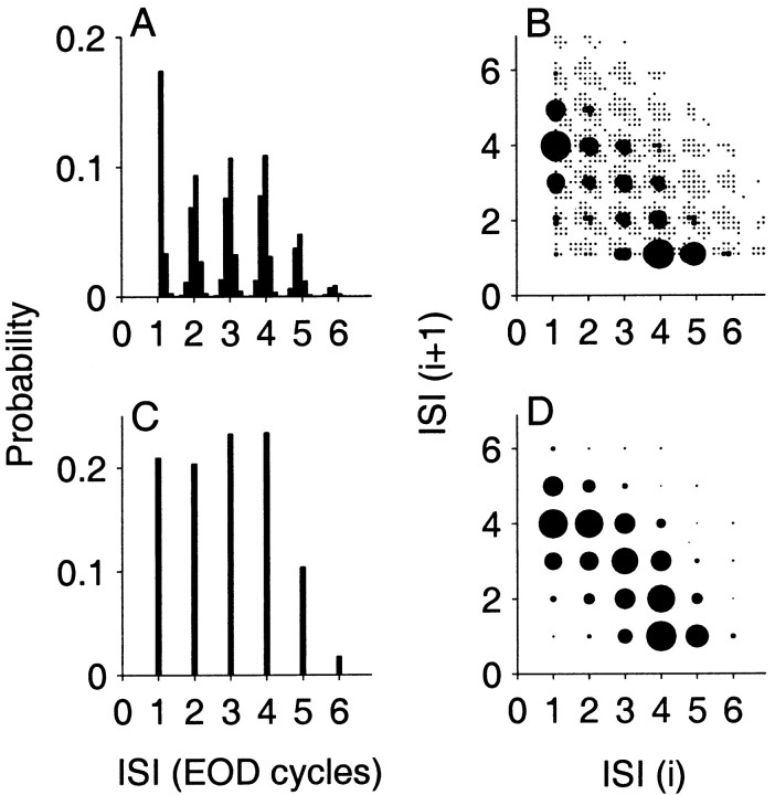
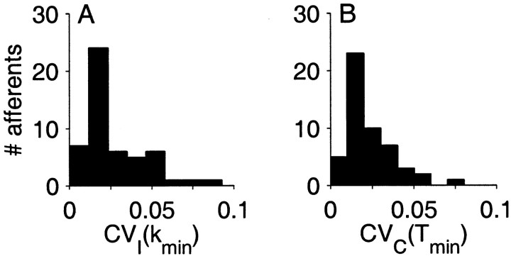
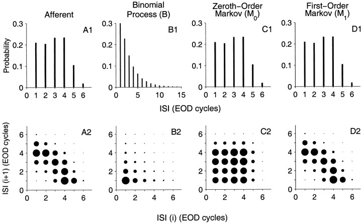
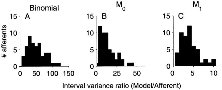
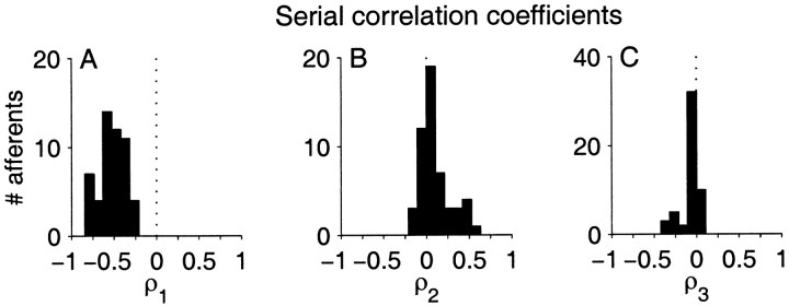
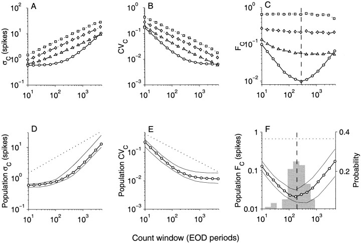
The ability of an animal to detect weak sensory signals is limited, in part, by statistical fluctuations in the spike activity of sensory afferent nerve fibers. In weakly electric fish, probability coding (P-type) electrosensory afferents encode amplitude modulations of the fish's self-generated electric field and provide information necessary for electrolocation. This study characterizes the statistical properties of baseline spike activity in P-type afferents of the brown ghost knifefish, Apteronotus leptorhynchus. Short-term variability, as measured by the interspike interval (ISI) distribution, is moderately high with a mean ISI coefficient of variation of 44%. Analysis of spike train variability on longer time scales, however, reveals a remarkable degree of regularity. The regularizing effect is maximal for time scales on the order of a few hundred milliseconds, which matches functionally relevant time scales for natural behaviors such as prey detection. Using high-order interval analysis, count analysis, and Markov-order analysis we demonstrate that the observed regularization is associated with memory effects in the ISI sequence which arise from an underlying nonrenewal process. In most cases, a Markov process of at least fourth-order was required to adequately describe the dependencies. Using an ideal observer paradigm, we illustrate how regularization of the spike train can significantly improve detection performance for weak signals. This study emphasizes the importance of characterizing spike train variability on multiple time scales, particularly when considering limits on the detectability of weak sensory signals.

Fig. 1.

Interval histograms of a P-type primary afferent fiber from the weakly electric fish Apteronotus leptorhynchus showing continuous-time (A, B) and discrete-time (C, D) representations.A, ISI histogram. Abscissa is multiples of EOD period (EOD frequency, f = 762 Hz). B, Joint distribution of adjacent intervals (joint interval histogram). Abscissa and ordinate are the i th and (i + 1) th ISIs in EOD periods, respectively, with symbol sizes proportional to probability of occurrence. Bin width is 180 μsec in A andB. Resampling the spike train at the EOD rate restricts the interspike intervals to integer values as shown in C (ISI histogram) and D (joint interval histogram). This afferent had a mean ISI of 2.9 EOD cycles and coefficient of variation (CV_I(1)) of 0.47. Subsequent analysis in this paper is restricted to the discrete-time representation, in which spike trains are sampled at the EOD rate.

Fig. 2.

Population summaries of ISI distributions (N = 52). A, Distribution of mean ISI ( $\overline{I}$₁). Abscissa is EOD cycles.B, Coefficient of variation of ISI (CV_I(1)).

Fig. 3.

SD (ς_I,left), coefficient of variation (CV_I,middle), and variance-to-mean ratio (F_I,right) of interval distributions. A–C, Representative fiber shown in Figure 1; D–F, medians of population (N = 52). Abscissa is the interval order. Symbols are: afferent data (○) and surrogate data sets from binomialB (□), zeroth-order Markov M₀(◊), and first-order Markov M₁ (▵) processes. In C, the afferent F_I curve exhibits a minimum for interval order k_min = 69 (vertical dashed line). In D–F, the afferent data (○) are medians for the population (N = 52) and the thin lines are upper and lower quartiles. Also shown are renewal processes (binomial, dotted; zeroth-order Markov,dash-dot). The histogram in F represents distribution of k_min in the afferent population (probability on right axis), with mean value of 42 (vertical dashed line).

Fig. 4.

Population summaries of coefficient of variation evaluated at the minimum in the variance-to-mean ratio curve.A, CV_I for intervals at order k = k_min. B, CV_C for spike counts at count window length T = T_min (see later in Results).

Fig. 5.

ISI histogram and joint interval histogram of the afferent spike train shown in Figure 1 (column A) and surrogate spike trains obtained from the afferent data (columnsB–D). A1–D1, Show the first-order ISI histograms I₁(j), and A2–D2 show the joint interval histogram I(j₁, j₂) of adjacent ISIs. Size of thecircle is proportional to joint probability. B, The binomial spike train matches the mean ISI $\overline{I}$₁, but it does not match either the ISI or joint ISI distributions. C, The zeroth-order Markov spike train (M₀) matches only ISI, but not the joint interval distribution. D, The first-order Markov spike train (M₁) matches both the ISI and joint ISI of the afferent spike train. ISI sequences for B and M₀ are renewal processes, whereas M₁ is a nonrenewal process.

Fig. 6.

Population summaries of the decrease in interval variance-to-mean ratio (F_I) observed in afferents when compared to F_I of the matched surrogate spike trains:A, binomial, B, zeroth-order Markov (M₀), and C, first-order Markov (M₁). Each histogram is the distribution of the ratio of the F_I(k_min) for surrogate divided by afferent. It measures the decrease in variability of intervals in afferents with reference to the surrogate spike train. Note different scales on abscissa.

Fig. 7.

Population summaries of serial correlation coefficients (ρ) of afferent ISI sequences. A–C, First three lags, ρ₁–ρ₃, respectively. The vertical dashed line is ρ = 0. The negative correlation for adjacent ISIs (ρ₁) reflects the strong long–short dependency in the ISI sequence.

Fig. 8.

Representative serial correlation coefficients (ρ_k, ordinate) for lags k = 1, … , 10 (abscissa). The ρ_kmeasure correlation between an ISI and the k th preceding ISI. A–C show ρ_k for three representative afferents (solid line) and for their matched surrogate first-order Markov spike train M₁(dash-dot line). Coefficients were tested against the null hypothesis that there was no correlation between the intervals at p = 0.01. The ρ_k which are significantly different from zero are indicated by *, whereas ○ indicates no significant correlation.

Fig. 9.

An illustration of how correlation analysis may fail to reveal memory effects in spike trains. A, Patterns of four adjacent ISIs (X, ?, ?, ?, Y) where “?” is any arbitrary value, were extracted from the ISI sequence S₁ for the afferent shown in Figure 1. The joint probability distribution of X and Y were estimated (probability is proportional to diameter of thecircle). The joint distribution suggests a very weak correlation between X and Y (see Results).B, Patterns of four adjacent ISIs (X, 2, 2, 2, Y) were extracted as in A. The distribution of X and Y is strongly influenced by conditioning it on the intermediate sequence (2, 2, 2). Serial correlation coefficients provide information from the distribution shown in A and not from the conditioned distribution shown in B. Hence, long-term memory effects may not be noticeable from correlation analysis.

Fig. 10.

Conditional entropy h_m for two representative afferent spike trains (solid line) as a function of order m. The mean h_m for 49 surrogate sequences which matched the data exactly up to order (m − 1) are also shown (□, dash line). Afferent h_m, which were significantly different from surrogate data are shown as *. Differences between afferent and surrogate data which were not significant are shown as ○. A, Afferent spike train that was described by a third-order Markov process. B, Spike train for which surrogate and afferent data sets had significantly different h_m for all orders tested. Testing terminated because of insufficient data. The order of the process was at least 5, i.e., the number represents only a lower-bound. See Table 1 for a summary of testing.

Fig. 11.

SD (ς_C,left), coefficient of variation (CV_C,middle), and variance-to-mean ratio (Fano factor F_C, right) of spike count distributions.A–C, Representative afferent (same afferent shown in Fig.3A–C). D–F, Medians of population (N = 52). Abscissa is count window duration T in EOD cycles. Symbols and layout follow Figure 3. InC, afferent F_C curve exhibits minima when count window T_min = 280 EOD periods (vertical dashed line). In D–F the dotted line is the median for surrogate binomial data with mean ISI equal to that of the afferent population. The histogram in F is the distribution of T_min in the afferent population, with mean value T_min = 233 EOD periods (vertical dashed line).

Fig. 12.

Population summaries of the decrease in count variance-to-mean ratio (Fano factor, F_C) observed in afferents when compared to F_C of the matched surrogate spike trains: A, binomial; B, zeroth-order Markov (M₀); and C, first-order Markov (M₁). Each histogram is the distribution of the ratio of the F_C(T_min) for surrogate divided by afferent. It measures the decrease in spike count variability in the afferents with reference to the surrogate spike trains. Note different scales on abscissa.

Fig. 13.

Signal detectability in afferent spike trains when spikes are added at random to baseline discharge. A, The detection strategy is based on a binary hypothesis test. In the presence of a signal, the baseline spike count distribution (Baseline) is shifted by an amount equal to the increase in number of spikes caused by signal (Baseline + Signal). A threshold (vertical dashed line) defines the probability of detection (gray area, P_d) and probability of false alarm (black area, P_fa). By constraining P_fa, P_d can be maximized.B, Spikes (abscissa) were added randomly to blocks of T = 100 EOD periods, and a signal detection algorithm (see Results) was given the task of determining whether signal was present subject to P_fa ≤ 0.001. Ordinate is P_d, and abscissa is number of extra spikes caused by signal. Detection experiments were simulated in afferent (○), and surrogate spike trains from binomial (B, □), zeroth-order Markov (M₀, ◊), and first order Markov (M₁, ▵) processes. For the afferent, signal detection performance at 90% (dashed line) is possible with as few as 2–3 spikes over the baseline of 35 spikes. Surrogate spike trains required more spikes to achieve the same level of performance (see Results).

References

1. Amassian VE, Macy J, Waller HJ, Leader HS, Swift M. Transformations of afferent activity at the cuneate nucleus. In: Gerard RW, Duyff J, editors. Information Processing in the Nervous System. Excerpta Medica Foundation; Amsterdam: 1964. pp. 235–254.
1. Baddeley R, Abbott LF, Booth MCA, Sengpiel F, Freeman T, Wakeman EA, Rolls ET. Responses of neurons in primary and inferior temporal visual cortices to natural scenes. Proc R Soc Lond B Biol Sci. 1997;264:1775–1783. - PMC - PubMed
1. Barlow HB, Levick WR. Changes in the maintained discharge with adaptation level in the cat retina. J Physiol (Lond) 1969a;202:699–718. - PMC - PubMed
1. Barlow HB, Levick WR. Three factors limiting the reliable detection of light by the retinal ganglion cells of the cat. J Physiol (Lond) 1969b;200:1–24. - PMC - PubMed
1. Bastian J. Electrolocation. I. how the electroreceptors of Apteronotus albifrons code for moving objects and other electrical stimuli. J Comp Physiol [A] 1981;144:465–479.
Publication types
LinkOut - more resources