Multiple scale dynamo

Abstract

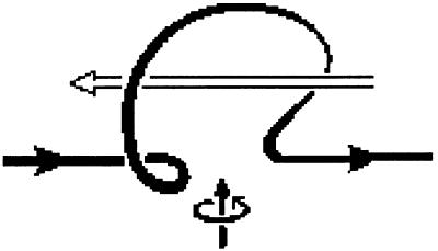
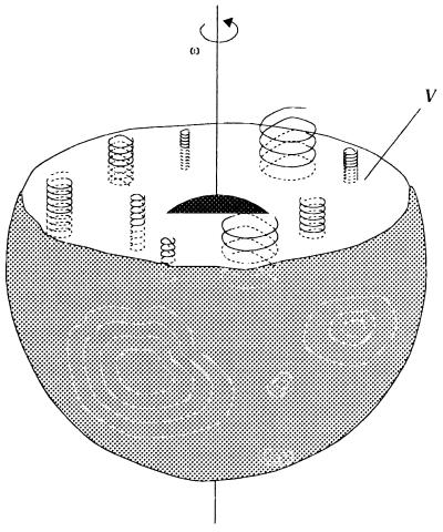
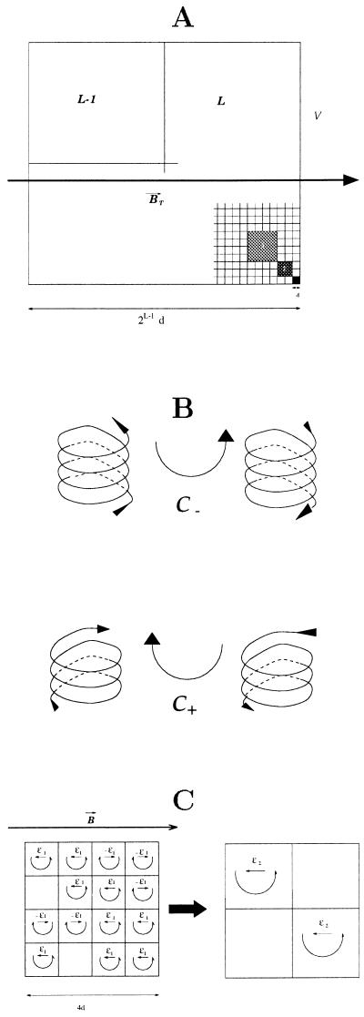
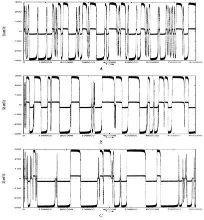
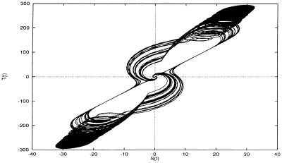
A scaling law approach is used to simulate the dynamo process of the Earth's core. The model is made of embedded turbulent domains of increasing dimensions, until the largest whose size is comparable with the site of the core, pervaded by large-scale magnetic fields. Left-handed or right-handed cyclones appear at the lowest scale, the scale of the elementary domains of the hierarchical model, and disappear. These elementary domains then behave like electromotor generators with opposite polarities depending on whether they contain a left-handed or a right-handed cyclone. To transfer the behavior of the elementary domains to larger ones, a dynamic renormalization approach is used. A simple rule is adopted to determine whether a domain of scale l is a generator--and what its polarity is--in function of the state of the (l - 1) domains it is made of. This mechanism is used as the main ingredient of a kinematic dynamo model, which displays polarity intervals, excursions, and reversals of the geomagnetic field.

Figure 1

A flux rope twisted into an Ω by a right-handed motion. The loop is accompanied by an electric current antiparallel to the magnetic field (14).

Figure 2

A representation of our model.

Figure 3

(A) The hierarchical model. The big square (𝒱) contains 2^2(ℒ−1) elementary squares of side d. (B) Conventional representation of right-handed and left-handed helical motion (cyclones) used in A and C. (C) Illustration of the scale transfer technique.

Figure 4

Examples of realizations of the process [𝒮(t), 𝒯(t)]. Values of the parameters are: c₀ = 10⁻², c₁ = 0.9, c₂ = 0, μ = 8 × 10⁻⁴, κ = × 10⁻², ζ = × 10⁻², ω = × 10⁻¹. (A) λ₁ = 7 × 10⁻¹², λ₂ = 8 × 10⁻⁷, λ₃ = 45. (B) λ₁ = 10⁻¹¹, λ₂ = 3 × 10⁻⁷, λ₃ = 50. (C) λ₁ = 1.5 × 10⁻¹¹, λ₂ = 10⁻⁷, λ₃ = 60.

Figure 5

Phase diagram [𝒮(t), 𝒯(t)] corresponding to Fig. 4A.

References

-
- Elsasser W M. Phys Rev. 1939;60:876–883.
- Takeuchi H, Shimazu Y. J Phys Earth. 1952;2:5–12.
- Parker E N. Astrophys J. 1955;122:293–314.
- Backus G. Ann Phys. 1958;4:372–447.
- Herzenberg A. Philos Trans R Soc London A. 1958;250:543–585.
LinkOut - more resources
Full Text Sources