Acoustic noise during functional magnetic resonance imaging

Abstract

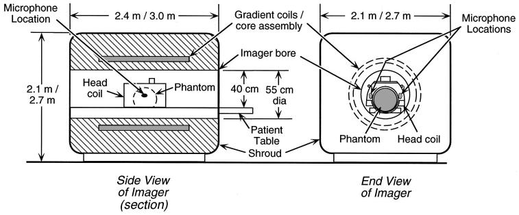
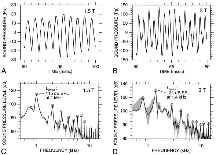
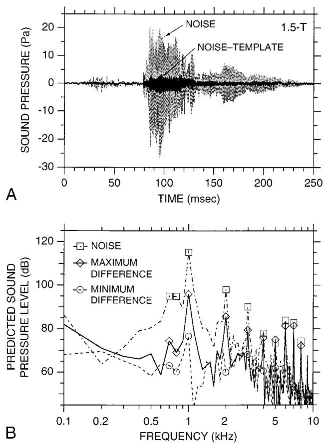
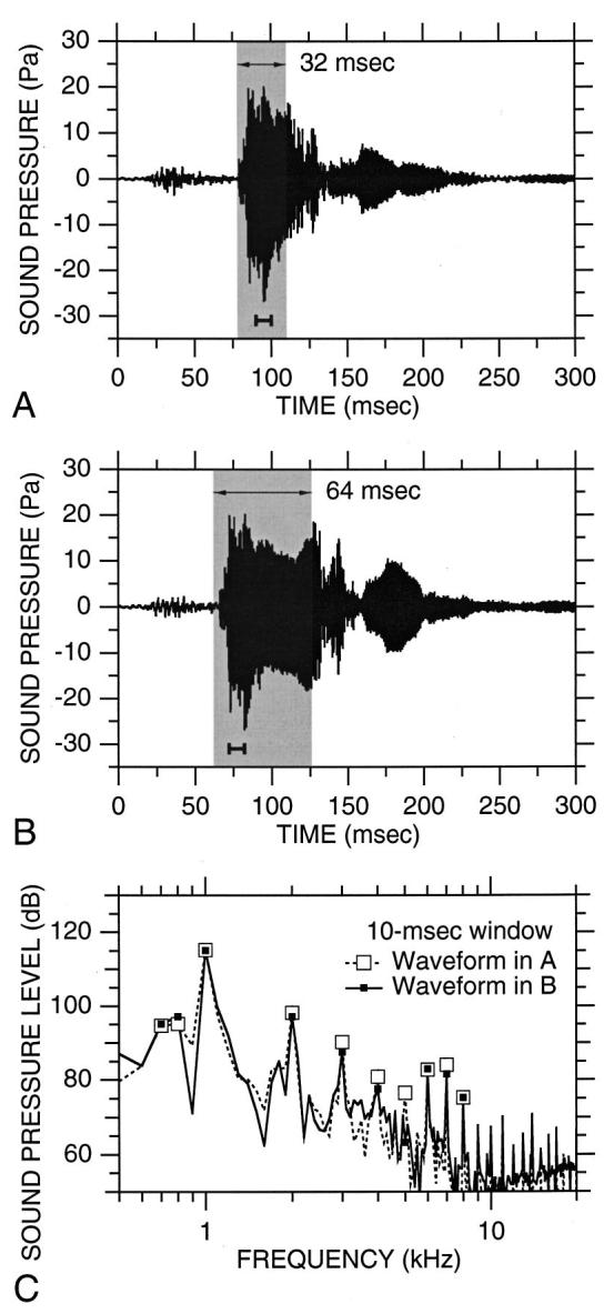
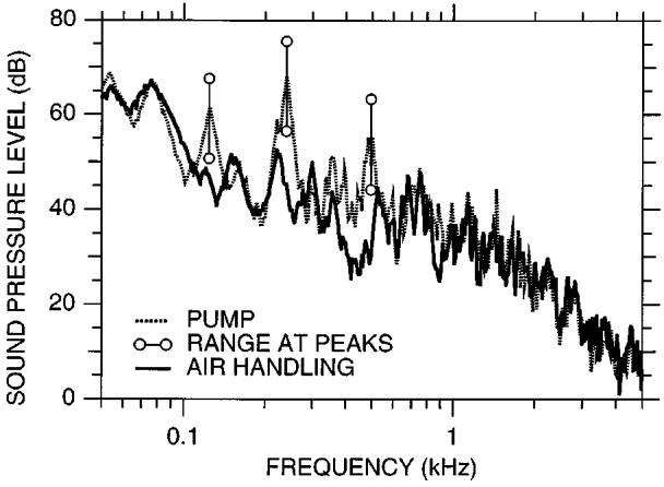
Functional magnetic resonance imaging (fMRI) enables sites of brain activation to be localized in human subjects. For studies of the auditory system, acoustic noise generated during fMRI can interfere with assessments of this activation by introducing uncontrolled extraneous sounds. As a first step toward reducing the noise during fMRI, this paper describes the temporal and spectral characteristics of the noise present under typical fMRI study conditions for two imagers with different static magnetic field strengths. Peak noise levels were 123 and 138 dB re 20 microPa in a 1.5-tesla (T) and a 3-T imager, respectively. The noise spectrum (calculated over a 10-ms window coinciding with the highest-amplitude noise) showed a prominent maximum at 1 kHz for the 1.5-T imager (115 dB SPL) and at 1.4 kHz for the 3-T imager (131 dB SPL). The frequency content and timing of the most intense noise components indicated that the noise was primarily attributable to the readout gradients in the imaging pulse sequence. The noise persisted above background levels for 300-500 ms after gradient activity ceased, indicating that resonating structures in the imager or noise reverberating in the imager room were also factors. The gradient noise waveform was highly repeatable. In addition, the coolant pump for the imager's permanent magnet and the room air-handling system were sources of ongoing noise lower in both level and frequency than gradient coil noise. Knowledge of the sources and characteristics of the noise enabled the examination of general approaches to noise control that could be applied to reduce the unwanted noise during fMRI sessions.

FIG. 1

Side view (left—in section) and end view (right) of a typical imager showing the gradient coils, bore, and location of microphones for noise measurements. The gradient coils and the cylindrical core on which they are wound surround the imager bore (the cylindrical opening through the center of the imager in which subjects lie during imaging). For noise measurements, a liquid-filled spherical plastic “phantom” (shown dashed in the side view) installed in a head coil was positioned where a subject’s head would be during brain imaging. The measurement microphones appear larger than their actual size (Shure: 4×6×10 mm, Knowles: 3×4×6 mm). Outer dimensions are given for the 1.5-T imager first, then the 3-T imager; bore diameter applies to both imagers.

FIG. 2

Acoustic noise measured over a time period including one image acquisition in the 1.5-T (A) and 3-T (B) imagers. Our standard imaging parameters were used (1.5 T: asymmetric spin echo, TE=70 ms, offset=-25 ms, field of view (FOV)=40×20 cm, TR=2 s, matrix size 128×64, slice thickness 7 mm; 3 T: spin echo, TE=35 ms, FOV=40×20 cm, TR=2 s, matrix size 128×64, slice thickness 5 mm). The imaged slice was in a plane that would be approximately parallel to the Sylvian fissure in a supine subject. A trigger pulse from the imager controller occurred at time=0. The rf transmitter was disconnected. The noise waveform for the remainder of the 2-s TR [i.e., time t>350 ms in (A), t>300 ms in (B)] resembles that for t<0 at this scale. Short horizontal bars below each waveform indicate waveform segments used in Fig. 3.

FIG. 3

Temporal and spectral characteristics of gradient coil noise.(A) and (B) 10-ms segments of the gradient noise in Figs. 2(A) and (B), respectively. In each case [(A) and (B)], the plotted segment corresponds to the 10-ms time window containing L_{f max}. These windows are indicated by the short thick bars below the waveforms in Fig. 2.(C) and (D) Spectra computed from the waveforms in (A) and (B), respectively (solid curves). Shading indicates the range of spectra seen for the other waveforms recorded during the same session [using our standard imaging parameters as in (A) and (B), and for the 10-ms time window corresponding to L_{f max}]. Squares (C) and triangles (D) indicate the spectral peaks that were tracked versus time as described in Sec. III A 3. The maximum spectral level L_{f max} is indicated. Spectral resolution: 100 Hz.

FIG. 4

Relationship between gradient coil noise and imaging pulse sequence (1.5 T). (A) Acoustic noise waveform from Fig. 2(A). Gray shading indicates when various gradients were on: (1) a brief “chemical saturation” gradient; (2) two slice-select gradients; and (3) readout and phase encode gradients. (B) Time course of the 1-kHz (thick solid curve), 2-kHz (thin solid curve and circles), and 700-Hz components (dashed curve) of the waveform in (A). Levels were computed from spectra of waveform segments obtained from a 10-ms rectangular window moved along the waveform in (A) at 5-ms intervals. Each data point in (B) corresponds to the center of the appropriate 10-ms window. Gray shading indicates gradient activity as in (A).

FIG. 5

Investigation of the repeatability of gradient coil noise (1.5 T). (A) A noise waveform before (light curve) and after (dark curve) an earlier noise waveform (i.e., a “template waveform”) was subtracted from it. The difference waveform shown (i.e., “noise-template”) had the greatest amplitude of all the difference waveforms calculated in our analyses. (B) Spectra computed over a 10-ms window from the noise waveform in (A) dot-dashed curve, squares), the maximum difference waveform in (A) (solid curve, diamonds), and the minimum difference waveform in our analyses (dashed curve, circles). In each case, the 10-ms window coincided with the waveform peak.

FIG. 6

Effect of doubling the duration of the readout and phase-encode gradient trains on the waveform and spectrum of acoustic noise (1.5 T). (A) Noise waveform from Fig. 4(A) obtained using our standard 1.5-T imaging parameters (matrix size 128×64). Gray shading indicates readout and phase-encode gradient activity. (B) Noise waveform obtained using the same parameters as in (A) except that the gradient duration was doubled (matrix size 256×128). (C) Spectrum of waveform in (A) (dashed line, open squares) and waveform in (B) (solid line, filled squares) computed over a 10-ms window coinciding with the peak noise [short bars under waveforms in (A) and (B)].

FIG. 7

Time-average spectra (unweighted) of noises produced by the combination of the 1.5-T imager coolant pump and the air handling system in the 1.5-T imager room (dotted curve) and the air-handling system alone (solid curve). For the peaks in the pump spectrum at 125, 240, and 490 Hz, the circles connected by vertical bars show the range of levels observed as a 100-ms time window was moved through the 1.7-s pump cycle.

References

1. ANSI . Specification for Sound Level Meters (amended) American National Standards Institute; New York: 1985. S1.4.
1. ANSI . Acoustical Terminology. American National Standards Institute; New York: 1994. S1.1.
1. ANSI . Measurement of Sound Pressure Levels in Air. American National Standards Institute; New York: 1995. S1.13.
1. Bandettini PA, Jesmanowicz A, Van Kylen J, Birn RM, Hyde JS. Functional MRI of brain activation induced by scanner acoustic noise. Magn. Reson. Med. 1998;39:410–416. - PubMed
1. Beranek LL. Acoustics. McGraw-Hill; New York: 1954. p. 481.
Publication types