Correlated firing in macaque visual area MT: time scales and relationship to behavior

Abstract

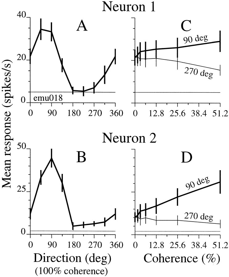
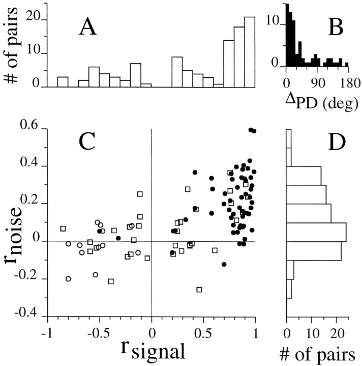
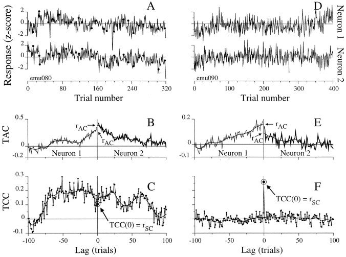
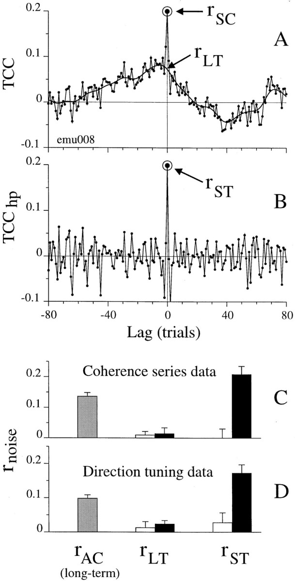
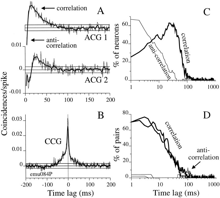
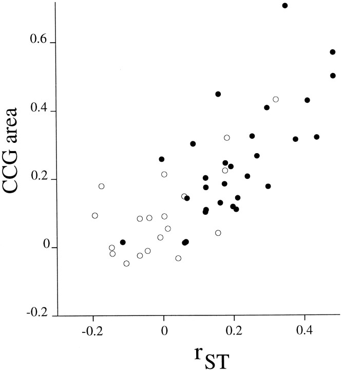
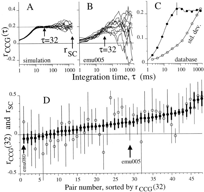
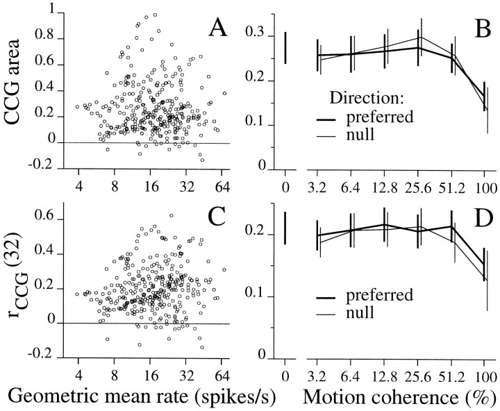
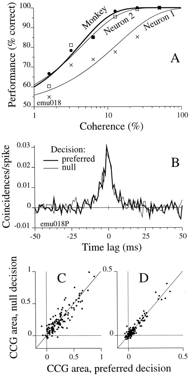
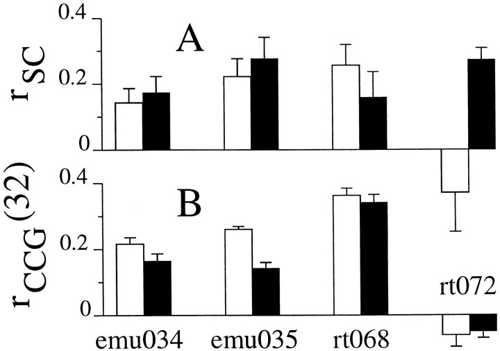
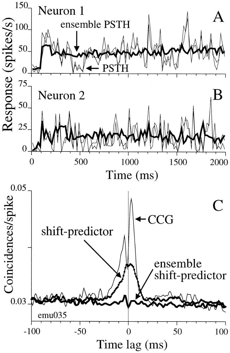
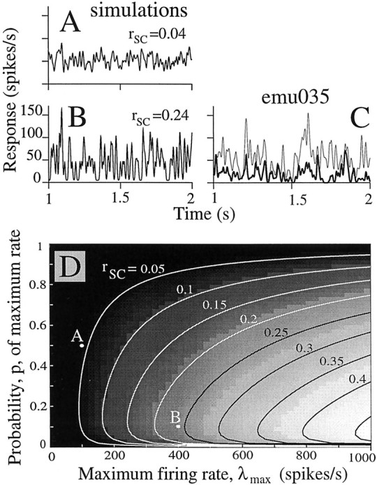
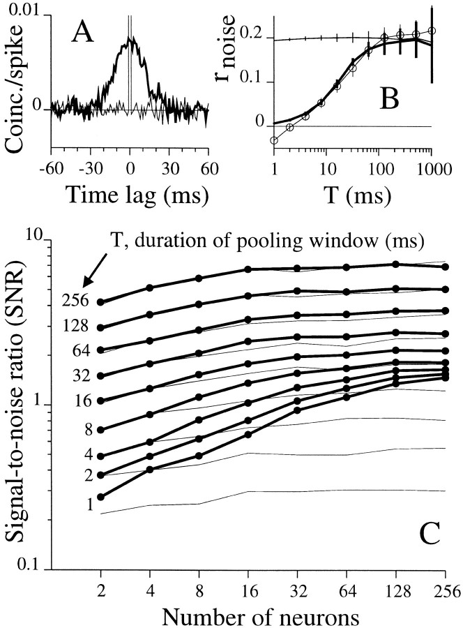
We studied the simultaneous activity of pairs of neurons recorded with a single electrode in visual cortical area MT while monkeys performed a direction discrimination task. Previously, we reported the strength of interneuronal correlation of spike count on the time scale of the behavioral epoch (2 sec) and noted its potential impact on signal pooling (Zohary et al., 1994). We have now examined correlation at longer and shorter time scales and found that pair-wise cross-correlation was predominantly short term (10-100 msec). Narrow, central peaks in the spike train cross-correlograms were largely responsible for correlated spike counts on the time scale of the behavioral epoch. Longer-term (many seconds to minutes) changes in the responsiveness of single neurons were observed in auto-correlations; however, these slow changes in time were on average uncorrelated between neurons. Knowledge of the limited time scale of correlation allowed the derivation of a more efficient metric for spike count correlation based on spike timing information, and it also revealed a potential relative advantage of larger neuronal pools for shorter integration times. Finally, correlation did not depend on the presence of the visual stimulus or the behavioral choice of the animal. It varied little with stimulus condition but was stronger between neurons with similar direction tuning curves. Taken together, our results strengthen the view that common input, common stimulus selectivity, and common noise are tightly linked in functioning cortical circuits.

Fig. 1.

Example of direction tuning curves and responses versus coherence for a pair of neurons recorded simultaneously. A and B show mean firing rate as a function of stimulus direction for the two neurons (pair emu018). Stimuli were 100% coherence moving dots. Error bars show ±1 SE.Thin, flat lines show spontaneous firing rate. C and D show mean firing rate as a function of coherence for preferred direction (90°, thick lines) and null direction (270°, thin lines) stimuli for the same neurons as A and B, respectively. Note that the minimum and maximum spike rates here do not reach those in A and B because 100% coherence was not included in these direction-discrimination experiments. Although some error bars are occluded at low coherence for null direction stimuli, they were roughly the same size as those for the preferred direction. A linear horizontal axis is maintained to emphasize the roughly linear relation between firing rate and coherence.

Fig. 2.

The joint distribution of signal and noise correlation for pairs of MT neurons. A, The marginal frequency distribution of r_signal for all pairs represented in C. B, The frequency distribution of Δ_PD (applicable to only those 69 pairs with both neurons directional) was similar to that reported by Albright et al. (1984) for pairs of MT neurons recorded successively at 50 μm intervals. Their study showed a second, small mode in the distribution for Δ_PD between 120 and 180°, corresponding to nearly opposite preferred directions for the two neurons. This mode was not readily apparent in our data; however, our sample size was smaller. From 104 pairs, 163 of 196 individual neurons (84%) were directional by the likelihood test described in Materials and Methods. C, Noise correlation is plotted against signal correlation for 103 pairs (direction tuning data). Squares indicate that at least one cell in the pair did not meet the directionality criterion (n = 34). Circles indicate directional pairs, andfilled circles (n = 57) indicate pairs with similar preferred directions, i.e., Δ_PD < 90°. For the 57 directional pairs with similar preferred directions, r_signal was typically high (median 0.86), and the mean r_noise value was 0.20 (SD 0.15), which was significantly greater than zero (p < 10⁻⁶; t test). The two filled circles in the top left quadrant represent pairs for which Δ_PD was only slightly <90° (87 and 83°) and for which peculiarities of the direction tuning curves caused r_signal to be negative. For directional pairs with Δ_PD ≥ 90°, r_noise = −0.02 (SD 0.09; n = 12; not different from zero; p = 0.59). For pairs with at least one nondirectional cell, r_noise = 0.06 (SD 0.15; n = 34; not different from zero; p = 0.11). D, Marginal frequency distribution of r_noise for all pairs represented in C.

Fig. 3.

The trial cross-covariance (TCC) can reveal the presence or absence of long-term correlation. A, The z -score normalized spike counts for all 320 trials are plotted in the order they occurred for two simultaneously recorded neurons (emu080). Spikes were counted during the 2 sec stimulus, but trials occurred on average 5 sec apart, so 100 trials represent ∼8.3 min. The dots show data points for preferred direction, 100% coherence stimuli to demonstrate how trials from one stimulus condition are interleaved among all others. B, Trial auto-covariance (TAC) plots are shown for the sequences from A, one on the left and one on the right side of lag 0 (the TAC is necessarily symmetrical about 0). Both have peaks of correlation around zero, indicating that the responsiveness of these neurons was not independent from trial to trial. The value at zero, 1 by definition, was omitted. The smooth line was used to estimate the value that the plot approached near the origin (arrows), referred to as r_AC or the long-term auto-correlation. C, The TCC is the cross-correlation of the sequences in A. TCC(0) (circled point) is the aggregate r_SC for the pair. For this pair, the value atTCC(0), 0.1, is associated with a peak that extends over lags of ±70 trials. The smooth line shows the TCC, with center value replaced (see Results), convolved with a Gaussian (SD 4 trials) and was used to estimate the long-term cross-correlation, r_LT. D, Traces similar to those in A, but for a different pair of neurons (emu090). Data are shown for the first 400 of 1320 trials. E, TACs for the traces in D. Both neurons show positive correlation around zero. F, The isolated peak at TCC(0)(circled point) for this pair indicates that correlation was predominantly short term, i.e., not associated with drifts in the responsiveness of the cells at time scales longer than the trial duration.

Fig. 4.

Noise correlation can be divided into short-term and long-term components. A, In the TCC (points connected by line segments, for pair emu008), the total noise correlation, r_SC, is the value at zero lag (circled point). The long-term correlation, r_LT, is the value of the smooth line (computed according to text, and Fig. 3C legend) at lag zero. B, For the same data as in A, the TCC_hp was computed after the z -scored spike counts were high-pass filtered. This eliminated the long-term correlation visible in A. The value at zero lag is taken to be the short-term correlation, r_ST. C, Database averages of correlation measures for coherence series data. Gray barshows long-term auto-correlation, r_AC, averaged across all individual neurons (n = 86). Long- and short-term cross-correlation, r_LT and r_ST, are shown for directional pairs with Δ_PD < 90 (black bars; n = 29) and other pairs (white bars; n = 19). Error bars show one SEM. D, The same measurements shown in C are shown here for direction tuning data from a larger set of pairs (n = 196 gray bars; n = 57 black bars; n = 47 white bars).

Fig. 5.

The time scale of spike train auto- and cross-correlation. A, ACG(τ) is plotted for two simultaneously recorded neurons (with ensemble shift-predictors subtracted). The thick line is a smoothed (Gaussian convolution, SD 2 msec) version of the raw ACG trace (thin line). The three horizontal lines show zero and ±3 SD of the noise (see Results). The top plot, ACG 1, has been shifted upward for clarity. B, CCG(τ) is plotted for the pair with ACGs that are shown in A. Again, a smoothed trace is superimposed, and horizontal linesindicate zero and ±3 SD of the noise. C, The fraction of neurons for which the ACGs were significantly (3 SDs) below (thin line) and above (thick line) the ensemble shift-predictor is plotted as a function of time lag (logarithmic axes). D, The fraction of pairs for which the CCG was significantly above (thick lines) and below (thin lines) the ensemble shift-predictor is plotted versus time lag. CCGs are two-sided, and results for negative time lags have been reflected onto positive time lags (yielding two traces at each thickness) for ease of comparison with the plot in C. Significant correlation occurs much more frequently for time intervals of several to tens of milliseconds than it does at or above 100 msec.

Fig. 6.

The area under the cross-correlogram peak is correlated with interneuronal correlation, r_noise. The area under CCG(τ) from τ = −32 to 32 msec and in excess of the ensemble shift-predictor is plotted against r_ST, an estimator of r_noise. The correlation coefficient for all points is 0.76 (p < 10⁻⁶; n = 48; coherence series data). A significant relationship also holds for the subset of 29 pairs for which Δ_PD < 90° (●) and for the remaining 19 pairs (○; see Results for statistics). The ordinate and abscissa have similar values here, but their units are not the same. A metric that estimates r_noise by appropriate normalization of the CCG peak area is demonstrated in Figure 7.

Fig. 7.

Computing r_CCG(τ) for simulated and neuronal data. A, r_CCG(τ) is plotted against integration time τ for 10 blocks of simulated pairs of spike trains in which the time scale and strength of correlation were known. (For each trial, 2 simulated spike trains were generated by selecting spike times independently and at random with probability 0.2 per spike from a Poisson spike train having mean rate 200 spikes per second. The rate is arbitrary and does not affect the results. The spike times in one of the resulting trains were jittered by adding a Gaussian random variable with mean zero and SD 4 msec. The resulting pairs of spike trains have r_noise = 0.2 and a time scale of correlation matching the Gaussian jitter.) For the simulated data, r_CCG(τ) approached the true value of r_noise once τ exceeded the time scale of correlation but became corrupted by noise as τ increased.Arrows indicate where r_CCG(32) and r_SC are read out. Here,r_CCG(32) = 0.200 SD 0.009, whereas r_SC = 0.197 SD 0.037 (n = 20). The ratio of SDs was 1:4. B, Results from an analysis similar to A but for 11 coherence levels for neuronal data (pair emu005). As in A, the curves rose from zero as τ increased but became highly corrupted by noise as τ exceeded 100 msec. For this pair, the width at one-half height of the CCG (data not shown) was 9 msec. C, The mean value of r_CCG(τ) across 29 pairs (averaged across all coherence levels for each pair with Δ_PD < 90°) is plotted as a function of τ in 1 msec steps (filled circles mark octave steps). Vertical bar indicates ±1 SE at τ = 64 msec. The SD of r_CCG(τ) is plotted at octave steps only (open circles connected by straight lines). The value of r_CCG reached an asymptote of ∼0.21 for τ around 30–100 msec, but the SD continued to increase with τ. D, r_CCG(32) (thick lines,filled circles) and r_SC (thin lines, open circles) for 48 pairs of neurons (coherence series data). Arrows indicate points corresponding to example pairs from B (emu005) and from Figure 3C (emu080). Points are sorted by increasing value of r_CCG. Vertical lines show ±1 SD (computed across coherence levels) and were always larger for r_SC.

Fig. 8.

CCG peak area and r_noise plotted as a function of geometric mean spike rate (GMSR) and motion coherence. A, The area of the CCG (minus the ensemble shift-predictor) integrated from τ = −32 to 32 msec is plotted as a function of GMSR for pairs of directional neurons with Δ_PD < 90°. Each point represents data for one coherence level from 1 of 29 qualified pairs. Pearson's correlation coefficient for this scatter was not significantly different from zero (r = −0.02; p = 0.65; n = 329). We chose our CCG normalization (Eq. 6) to realize this empirical observation. For individual pairs, 3 of 15 negative relationships and 6 of 14 positive relationships were significant (p < 0.05). B, Mean CCG area (±32 msec) averaged over the same 29 pairs as in A is plotted for preferred (thick line) and null (thin line) motion as a function of coherence (there are typically 24–29 pairs per point because some pairs were not tested at all coherence levels).Vertical bars show ±1 SEM. Values remained relatively constant except for a 43% reduction at 100% coherence compared with the average across all lower coherence stimuli (preferred and null directions combined). C, A measure of r_noise, here r_CCG(32), is plotted against GMSR for the same set of pairs. There is a small overall positive correlation with mean spike rate (r = 0.14; p = 0.01; n = 329). For individual pairs, 1 of 12 negative and 6 of 17 positive relationships were significant. D, Like CCG area, the r_noise measure varies little with motion direction and coherence except at 100% coherence where it dropped by 32% relative to the average across all lower coherence levels (preferred and null directions combined). As in B, typically 24–29 pairs contributed data to each point.

Fig. 9.

Psychophysical and neuronal performance. A, The monkey's performance (filled circles) and the neuronal performance for neuron 1 (×'s) and neuron 2 (squares) are plotted as a function of motion coherence (logarithmic axis) for the same pair of neurons as in Figure 1. The lines show fits to Equation 2. The thick line is for the monkey's psychophysical responses. B, An example of average CCGs for preferred (thick lines) and null (thin lines) direction decisions. CCGs for coherence levels of ±6.4, ±3.2, and 0% were averaged together; other coherence levels did not have a sufficient number of choices in each direction. C, The area under the CCG between −32 and 32 msec and in excess of the shift-predictor for null decisions is plotted versus that for preferred decisions. Each point (n = 137) shows data for a particular coherence level and direction, so there are multiple points per neuronal pair (n = 35). D, For the same data set as in C, the comparison of CCG area is made for a narrower integration region, from −2 to 2 msec. Results in B–D reflect a lack of correlation between perceived direction of motion and the magnitude of synchronous activity in the population of neurons that prefer the perceived direction.

Fig. 10.

A comparison of interneuronal correlation strength for stochastic versus replicate stimuli. A, r_SC is plotted for four pairs tested with both ensemble (white bars) and replicate (black bars) stimuli. No significant change was observed for the first three pairs. For the fourth pair, the responses to replicate stimuli had a large long-term component of correlation because of drifts in firing rate during the experiment (r_LT = 0.27, r_ST = 0.02). Error bars show SE. B,r_CCG(32) is shown for the same four pairs. In the first three cases, r_CCG(32) was less for replicate stimuli. The difference was significant for emu035(see Results). Lower values for replicate stimuli (black bars) were consistent with the reduction in the CCG peak that occurred when the true shift-predictor (Fig. 11C) was subtracted. Cases emu034 and emu035 were based on coherence series data; rt068 and rt072 were based on direction tuning data (c = 100%). Forrt072, the low r_noise value was consistent with Δ_PD > 90°.

Fig. 11.

Comparing PSTHs and shift-predictors for responses to ensemble and replicate stimuli for pair emu035. A, PSTHs (bin size 20 msec) for neuron 1 averaged across 60 trials of different 0% coherence stimuli (thick line, ensemble stimuli) and averaged across 30 trials of one particular 0% coherence stimulus (thin lines, replicate stimuli, broken into 2 groups of 15 trials to demonstrate that the modulation is reproducible). B, Similar to A, but for the simultaneously recorded responses of neuron 2. C, The raw CCG (without the shift-predictor subtracted; thin line) is plotted for comparison against the ensemble shift-predictor (thick line) and the actual shift-predictor (points) computed from responses to replicate stimuli. Plots show averages across 13 stimulus conditions ranging from 0 to 51.2% coherence, preferred and null directions. The shift-predictor accounts for roughly half of the area of the CCG peak. It is worth noting that the raw CCG for ensemble stimuli does not differ on average from that for replicate stimuli because both result from cross-correlation of simultaneous responses to stimuli with the same underlying statistics; therefore, only one trace markedCCG is shown here. Of course, any particular CCG from repeats of one replicate stimulus will deviate from the average ensemble CCG, but if raw CCGs from many different replicate stimulus sets are averaged together, they will approach the raw ensemble CCG. This is not true for shift-predictors, as seen here, because they are based on responses from non-simultaneous trials.

Fig. 12.

Modeling the interneuronal correlation caused by stimulus variation for a pair of identical neurons. A, Simulated time-varying instantaneous mean firing rate for p = 0.5, λ_max = 100 spikes/sec, λ_min = 5 spikes/sec (smoothed with Gaussian SD 4 msec to achieve a realistic temporal resolution). The single line represents the PSTHs for two identical neurons in an ideal pair. See Appendix for a description of the model. B, Similar to A, but p = 0.1, λ_max = 400 spikes/sec. C, PSTHs for pairemu035 for comparison to the simulations. The PSTHs for neuron 1 (thin line) and neuron 2 (thick line) represent a segment of the same data shown by the pairs of thin lines in Figure 11, A and B, but are smoothed like the simulation traces in A and B here. D, For our model, r_SC is plotted as a function of all values of p and λ_max (see Eq. 39). Points A and B mark parameters used to generate traces in Aand B. Black shading indicates low correlation,white indicates high correlation. Values are given for thecontour lines.

Fig. 13.

Changes in r_noise and SNR as a function of pooling time, T. A, CCGs of simulated spike trains are plotted for two hypothetical neuronal populations, one with a realistic time scale of pair-wise correlation (thick line, approximates a Gaussian of SD 8 $\sqrt{2}$ msec) and one with instantaneous correlation (thin line, peak at zero is truncated). Simulation method is described in the legend for Figure7A. B, For pairs from the two hypothetical populations, r_noise was computed as a function of T, the period in which spikes would be counted to form a population response. For instantaneous correlation, r_noise was constant (here 0.2) for all integration times (thin line). However, for broad correlation (thick line), r_noise was near zero for short T and increased to the veridical value as T became large relative to the time scale of correlation. Results for the simulated broad correlation were comparable to those for our neuronal data (open circles; r_noise averaged across 29 neuronal pairs that were directional and had Δ_PD < 90°, coherence series data). The negative value at 1 msec for the neuronal data results from limitations in recording two nearly simultaneous action potentials using one electrode. Error bars for the model show SD across 10 blocks of 200 trials (mean firing rate 40 spikes per second). Error bars are smaller for smaller window sizes because, for example, there are 1000 T = 1 msec windows for each T = 1000 msec window. C, Pooled signals (sums of spike counts) from the hypothetical populations were compared in terms of their SNR (Eq. 10) as a function of neuronal pool size for time windows of various duration. For instantaneous correlation, the SNR curves (thin lines) had the same shape for all T but were scaled by $\sqrt{2}$ when T doubled. For the more realistic case of broad correlation, however, the SNR curves (thick lines) increased more steeply with pool size for short T because r_noise was less for short T (as shown by the thick line in B).

References

1. Abbott LF, Dayan P. The effect of correlated variability on the accuracy of a population code. Neural Comput. 1999;11:91–101. - PubMed
1. Abeles M. Local cortical circuits: an electrophysiological study. Springer-Verlag; Berlin: 1982.
1. Aertsen AMHJ, Gerstein GL, Habib MK, Palm G. Dynamics of neuronal firing correlation: modulation of “effective connectivity.”. J Neurophysiol. 1989;61:900–917. - PubMed
1. Albright TD, Desimone R, Gross CG. Columnar organization of directionally selective cells in visual area MT of the macaque. J Neurophysiol. 1984;51:16–31. - PubMed
1. Arieli A, Sterkin A, Grinvald A, Aertsen A. Dynamics of ongoing activity: explanation of the large variability in evoked cortical responses. Science. 1996;273:1868–1871. - PubMed
Publication types
MeSH terms
LinkOut - more resources