Spatial structure of cone inputs to color cells in alert macaque primary visual cortex (V-1)

Abstract

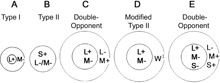
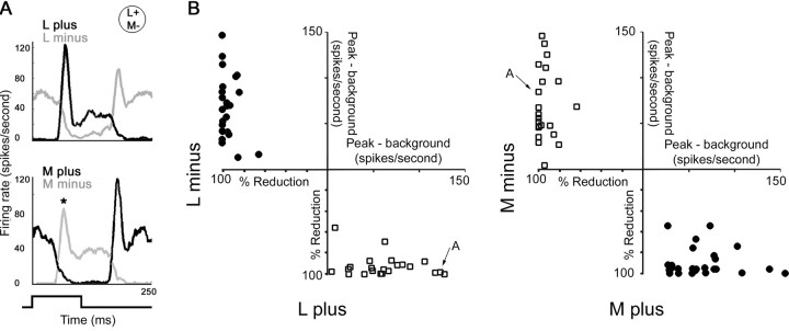
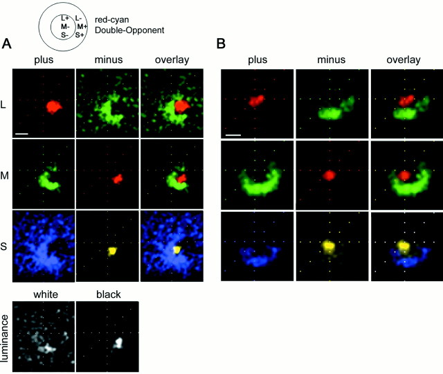
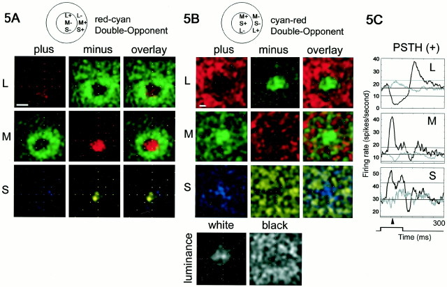
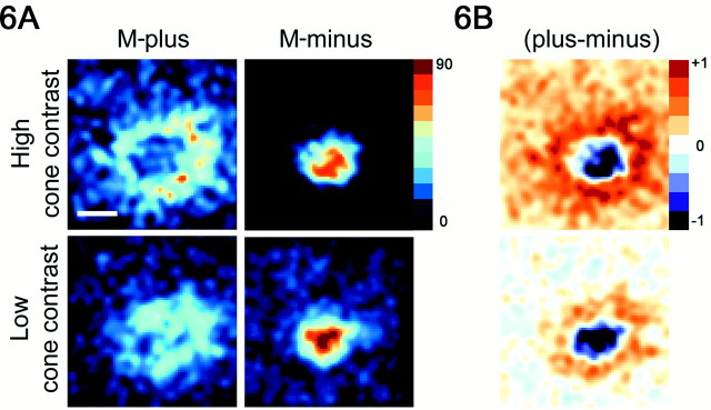
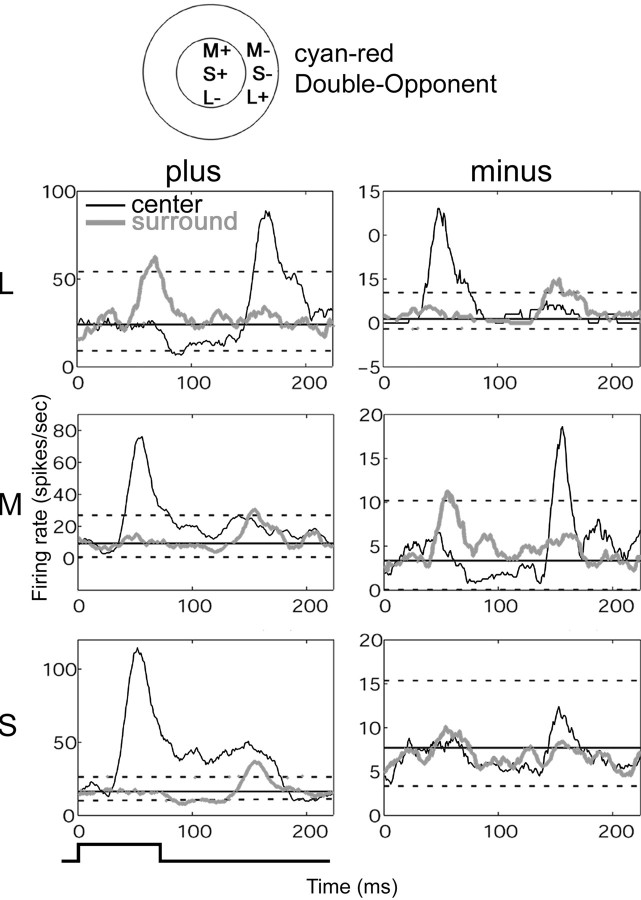
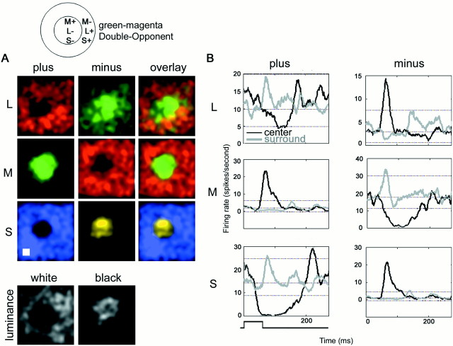
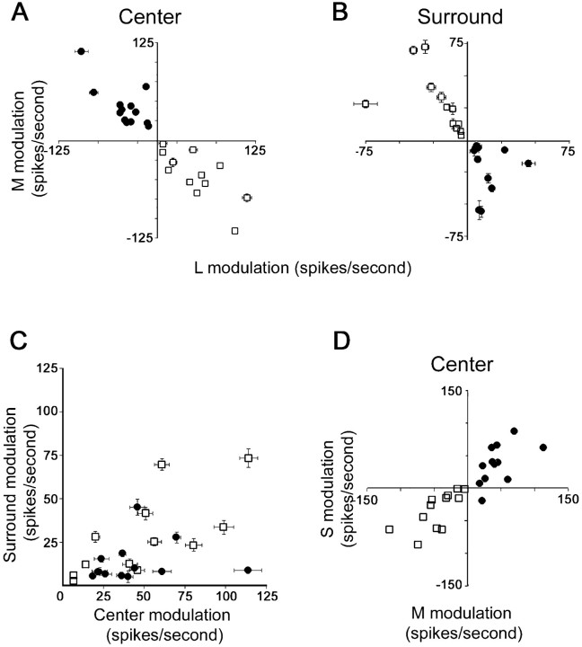
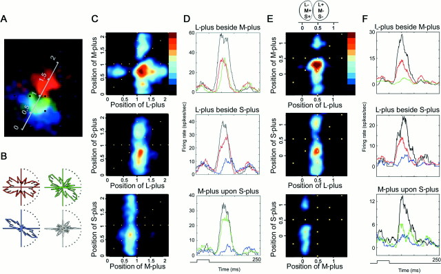
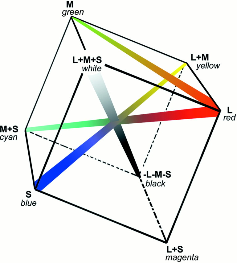
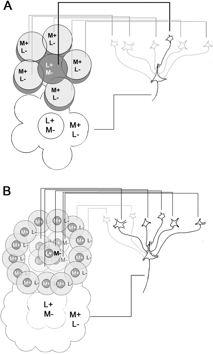
The spatial structure of color cell receptive fields is controversial. Here, spots of light that selectively modulate one class of cones (L, M, or S, or loosely red, green, or blue) were flashed in and around the receptive fields of V-1 color cells to map the spatial structure of the cone inputs. The maps generated using these cone-isolating stimuli and an eye-position-corrected reverse correlation technique produced four findings. First, the receptive fields were Double-Opponent, an organization of spatial and chromatic opponency critical for color constancy and color contrast. Optimally stimulating both center and surround subregions with adjacent red and green spots excited the cells more than stimulating a single subregion. Second, red-green cells responded in a luminance-invariant way. For example, red-on-center cells were excited equally by a stimulus that increased L-cone activity (appearing bright red) and by a stimulus that decreased M-cone activity (appearing dark red). This implies that the opponency between L and M is balanced and argues that these cells are encoding a single chromatic axis. Third, most color cells responded to stimuli of all orientations and had circularly symmetric receptive fields. Some cells, however, showed a coarse orientation preference. This was reflected in the receptive fields as oriented Double-Opponent subregions. Fourth, red-green cells often responded to S-cone stimuli. Responses to M- and S-cone stimuli usually aligned, suggesting that these cells might be red-cyan. In summary, red-green (or red-cyan) cells, along with blue-yellow and black-white cells, establish three chromatic axes that are sufficient to describe all of color space.

Fig. 1.

Diagrams of the receptive fields of color-responsive cells. A plus indicates excitation by the given cone, and a minus indicates suppression.A, A Type I cell. Type I cells, which are the major cell class in the parvocellular layers of the LGN, have opponent chromatic inputs that are not completely overlapping. Type I cells have very small receptive field centers, often fed by a single cone.B, A blue-on/yellow-off Type II cell. Type II cells, found in the koniocellular layers of the LGN, have opponent chromatic inputs that are spatially coextensive. The centers of Type II cells (scaled for eccentricity) are much larger than those of Type I cells and comprise many cones. Type II cells are excited by one color and suppressed by another. This “blue-on” cell would be excited by blue light and suppressed by yellow light. Blue–yellow Type II cells are well described; red–green Type II cells remain to be documented conclusively. C, A red-on center Double-Opponent cell. Double-Opponent cells have receptive fields that are both chromatically opponent and spatially opponent. The existence of Double-Opponent cells in the monkey visual system is controversial. D, A modified Type II cell. This class is thought by some to exist in V-1 and represent the major class of color-coding cells.W^I indicates suppression of center response by all cones. E, An example of the organization of color cells reported here [see Note concerning S cone input (Materials and Methods) and Do red–green cells receive S-cone input? (Results) for a discussion of the validity of the S-cone input].

Fig. 2.

Gun luminance function. The luminance of the computer monitor (in candelas per square meter) was measured separately for each gun. Crosses, Red gun; circles, green gun; triangles, blue gun. These values were fit by polynomials (lines). This enabled me to normalize the gun values, which was necessary in generating the cone-isolating stimuli (see Materials and Methods).

Fig. 3.

Modulation of cell activity in response to flashes of cone-isolating light presented in the center of color cell receptive fields. A plus stimulus selectively increased the activity of a given class of cones but maintained constant activity of the other two classes. A minus stimulus selectively decreased the activity (see Materials and Methods and Table 1). A, PSTHs for an L+/M− centered cortical cell. The cell was excited by the L-plus stimulus (top plot, black trace) and suppressed by the L-minus stimulus (top plot,gray trace); it also gave opponent responses to the M-plus stimulus (bottomplot,black trace) and the M-minus stimulus (bottom plot, gray trace). This cell gave opponent responses to the L-plus and M-plus stimuli, identifying it as a color cell. A luminance cell would respond with the same sign (excitation or suppression) to L- and M-plus stimuli. The stimulus was a ∼1 × 1° square centered on the receptive field; it was on for 100 msec (indicated at bottom). The peak response to M-minus (asterisk) was used as a measure of the full extent of suppression by M-plus (see Quantification of double opponency in Results). B, Responses determined from PSTHs for 47 color cells screened as in A. Modulation in response to L-plus and L-minus (left graph) and in response to M-plus and M-minus (right graph) is shown: red-on-center cells (open squares) and green-on-center cells (filled circles). The response was categorized as suppression (e.g., response to L-minus in A) or excitation (e.g., response to L-plus in A). Suppression was then quantified as a percentage of reduction of background, in which background was calculated based on the first 40 msec of the PSTH. Excitation was quantified as (peak − background) (in spikes per second). The cell whose PSTH is given in A is identified.

Fig. 4.

Receptive fields of two red-on-center/green-on-surround Double-Opponent cells recorded in alert macaque V-1. A, A small patch of cone-isolating light was flashed at random locations in and around the receptive field; response maps were generated using an eye-position-corrected reverse correlation technique (see Materials and Methods). The maps reflect the average stimulus position that preceded each spike and are corrected for eye position and for the visual latency. L-plus, M-plus, and S-plus, left column; L-minus, M-minus, and S-minus,middle column; and overlay, right column. The background firing rate has not been subtracted from these maps.Black in these maps represents a firing rate of zero spikes per second; more intense responses are represented as more saturated colors. Peak firing rates (spikes per second) were as follows: L-plus, 62; L-minus, 20; M-plus, 35; M-minus, 47; S-plus, 16; S-minus, 71; white, 21; black, 27. Stimulus size was 0.4 × 0.4°. This cell was 4° peripheral. Scale bar (in Aand B), 0.5°. The coloring of the maps does not match that of the stimuli. The L-plus and M-minus maps are coloredred because the stimulus in both cases appears red; the L-plus stimulus is a bright red (on a dark bluish-green), and the M-minus is a dark bluish-red (on a bright green background).B, Response maps for a second red-on-center Double-Opponent cell. Peak firing rates (spikes per second) are as follows: L-plus, 67; L-minus, 45; M-plus, 77; M-minus, 57; S-plus, 23; S-minus, 30. This cell was 5° peripheral. Stimulus size was 0.4 × 0.4°.

Fig. 5.

Response maps for a strongly Double-Opponent cell (A) and a weakly Double-Opponent cell (B). Conventions as in Figure 4.A, Peak firing rates (spikes per second) were as follows: L-plus, 53; L-minus, 37; M-plus, 55; M-minus, 71; S-plus, 10; S-minus, 54. B, Peak firing-rates (spikes per second) were as follows: L-plus, 23; L-minus, 43; M-plus, 41; M-minus, 12; S-plus, 53; S-minus, 37; white, 32; black, 22. Both cells were 5° peripheral; stimuli were 0.4 × 0.4°. Scale bar (inA and B), 0.5°. C, Responses were determined from the reverse correlation data by selecting segments of the spike train corresponding to presentations of plus stimuli in the center (black traces) and surround (gray traces) of the cell whose response maps are given in B. Stimulus duration was 100 msec (indicated atbottom). The response maps in Bcorrespond to the response of a cell between 50 and 70 msec after the onset of the stimulus (arrowhead). One SD above and below the mean background firing rate is given for reference.

Fig. 6.

Comparison of response maps generated using high cone-contrast stimuli and low cone-contrast stimuli. A, Response maps for the red-on-center cell shown in Figure5A were generated using both high cone-contrast stimuli (top panels) and low cone-contrast stimuli (bottom panels). Only the maps for M-plus and M-minus are shown. The responses are color-coded with a linear color scale bar:black represents zero spikes per second, and thedarkest red represents 90 spikes per second. All maps reflect responses after the same number of stimulus presentations. Scale bar, 0.5°. B, Difference maps between the minus and plus response maps. White represents no difference between the minus and plus maps. Note that the region surrounding the receptive field for the low cone-contrast stimulus is approximatelywhite, reflecting the constant background activity between the plus and minus conditions. This is not the case for the high cone-contrast stimuli, which have different adapting backgrounds and therefore different background firing rates for the plus and minus conditions.

Fig. 7.

Temporal organization of a cyan–red Double-Opponent cell. Poststimulus time histograms corresponding to stimulation in the center (black traces) and surround (gray traces) for the plus stimuli (left plots) and minus stimuli (right plots) generated from the reverse correlation data (conventions as in Fig.5C). A normalized mean firing rate was calculated based on the first 40 msec (straight solid lines); one SD below and two above are plotted as reference (straight dotted lines). The cell was excited when an M-plus stimulus was presented in the center (middle left plot, black trace) and suppressed when an L-plus stimulus was presented in the center (top left plot, black trace). Inverse responses were obtained in the surround. The off-discharge after release of suppression is a useful indicator of the preceding suppression in situations in which the background activity was so low that suppression is not obvious (e.g., M-plus surround, middle left plot, gray trace). In addition to a strong surround response, this cell exhibited strong S-plus responses that coincided in space and sign with the M-plus responses; this is summarized in the diagram at top. Stimulus duration, 73 msec, indicated at the bottom left; stimulus size, 0.9 × 0.9°. This cell was 3° peripheral.

Fig. 8.

Response maps and temporal organization for a green–magenta Double-Opponent cell. A, Response maps to the six stimuli conditions; conventions as in Figure 4. Stimulus size was 0.4 × 0.4°, shown at the bottom left. Unlike the other cells shown, the S-cone input in this cell aligns in space and sign with the L-cone input, justifying a description of this cell as green–magenta (in which magenta is red plus blue).B, Temporal organization of the response of the cell whose spatial response maps are shown in A. Conventions as in Figure 5C. Center, black traces; surround, gray traces; plus stimuli, plots on the left; minus stimuli, plots on the right. One SD below and two above the mean firing rates are shown for reference. Stimulus duration is indicated at the bottom left.

Fig. 9.

Quantification of cone inputs to cortical color cells. A, Responses were determined from the reverse correlation data by selecting segments of the spike train corresponding to stimulus presentations in the center. The stimuli often reduced the firing of the cells to zero spikes per second, making it impossible to directly measure the full extent of the suppression. To find a more meaningful measure of suppression (rather than reduction of background), I assumed that the suppression was equal in magnitude but opposite in sign to the excitation produced by the opposite contrast stimulus (see Results). For example, for the red-on-center cell shown in Figure 3A, the suppression by the M-plus stimulus would be equal, but opposite in sign, to the excitation by the M-minus stimulus (asterisk in Fig. 3). The responses of the cells to M modulation (ordinate) is plotted against the response to L modulation (abscissa). All green-on-center cells (filled circles) fall in quadrant 2, whereas all red-on-center cells (open squares) fall in quadrant 4, showing that the centers were chromatically opponent. B, Surround responses were extracted from the reverse correlation data, as in A. The green-on-center cells and the red-on-center cells swap quadrants. This shows that the chromatic opponency of the surrounds of both populations of cells was opposite that of their centers.C, Surround responses were generally weaker than center responses. For green-on-center cells (filled circles), the L-plus surround response is plotted against the M-plus center response. For red-on-center cells (open squares), the M-plus surround response is plotted against the L-plus center response. D, Red–green cells were often modulated by the S-cone-isolating stimulus. The response to presentation of the S-cone-isolating stimulus in the center of the receptive field (ordinate) is plotted against the response the M-cone-isolating stimulus (abscissa). In all plots, the average background activity (see Fig. 3) was subtracted from the peak responses.

Fig. 10.

Interaction between the cone inputs of two oriented Double-Opponent cells. A, Reverse correlation map for the three plus stimuli for one cell; conventions as in Figure4. The scale bar (in degrees) is placed perpendicular to the orientation preference of the cell. The M-plus response is between 0.5 and 1°, and the L-plus response is between 1 and 1.5°. Stimulus size, 0.3 × 0.3°. B, Orientation tuning was generated using flashed oriented bars of cone-isolating stimuli and white. The cell responded poorly to white (white plot). The orientation tuning to L-plus bars (red plot), M-plus bars (green plot), and S-plus bars (blue plot) is reflected in the orientation of the subregions of the response map shown in A. C, Responses to simultaneously presented pairs of optimally oriented cone-isolating bars (see Cone interactions in Results). Cell response is represented by the graded color scale, with black being 0 anddark red being 65 spikes per second. The axes of the plots are the same as the scale bar in A. Hence, in thetop panel of C, the L-plus response is between 1 and 1.5°, and the M-plus response is between 0.5 and 1°. The x = y diagonal denoted byyellow dots represents the position across the receptive field at which the bars overlapped. The response is decreased along this diagonal for the L-plus versus M-plus plot (top), similarly for the L-plus versus S-plus plot (middle), but the response is increased along thisdiagonal for the M-plus versus S-plus plot (bottom). As one would predict based on the response maps shown in A, the response is maximal when L-plus bars are placed adjacent to M-plus bars. This is indicated by thedark red in the top plot at the coordinates (1.25, 0.75). D, PSTHs corresponding to the peak responses in C. Black lines are the PSTHs to optimally placed pairs of bars; L-plus and M-plus bars are adjacent to each other (top panel), L-plus and S-plus bars are adjacent to each other (middle panel), and M-plus and S-plus bars are superimposed (bottom panel). Colored linesrepresent the response of the cell to the optimal placement of a single bar: L-plus, red lines; M-plus, green lines; S-plus, blue lines. Stimuli were presented for 48 msec, shown at the bottom. This cell was 5° peripheral. E, Interaction maps for a second cell. The stimulus range (in degrees) forms the axes of the interaction plots and is also indicated below the diagram of the spatial organization of the receptive field (above top panel). Along the stimulus range, the M/S-plus-on subregion is ∼0.25°, and the L-plus-on subregion is ∼0.5°. The color scale bar (top panel) indicates the cell response; peak response (dark red) is 30 spikes per second. F, PSTHs corresponding to the peak responses inE; conventions as in D, above. This cell was 4° peripheral. Stimulus size, 0.75° × 0.2°.

Fig. 11.

The results presented here suggest that the cortex exhibits a single red–green axis: the responses of red–green cells to an L-cone-isolating stimulus are well predicted by their responses to an M-cone-isolating stimulus (Fig. 9A,B). In the cortex, this red–green axis is presumably accompanied by a blue–yellow axis [S vs (M + L)] and a luminance axis (see Discussion). These three axes are sufficient to describe all of color space, represented here as a cube. In the present study, the majority of L versus M cells responded to an S-cone stimulus, and these responses aligned in space and sign with responses to the M-cone stimulus (Fig. 9D). If these responses reflect a genuine S-cone input (and not an artifact of longitudinal chromatic aberration; see Note concerning S-cone stimuli in Materials and Methods), then these cells would be better described as L versus ½(M + S), or red–cyan. The color names provide a useful mnemonic and seem justified. A stimulus that selectively increases the activity of M- and S-cones appears cyan; similarly, one that increases the activity of the L-cones appears red. S, Blue–violet;L+M, yellow.

Fig. 12.

Models describing the hypothesized inputs into a Double-Opponent cell. A, One red-on/green-off Type II cell feeds the center of the Double-Opponent cell. The surround is fed by Type II cells of opposite configuration, green-on/red-off (shown ingray) (adapted from Michael, 1978). Although early studies suggest the existence of red–green Type II cells in the LGN, subsequent investigators have not found them. Thus, although LGN Type II cells may be involved in forming blue–yellow cortical Double-Opponent cells, an alternative model is required for the formation of cortical red–green Double-Opponent cells. For example,B, a group of parvocellular LGN Type I cells whose receptive field centers are dominated by the same cone class (in this case L), could feed the center, whereas the surround could be fed by Type I cells of the opposite configuration (2 cells are shown ingray). A cortical red–green Type II cell would result if the surround were insignificant.

References

1. Albers J. Interaction of color, pp 20–21. Yale UP; New Haven, CT: 1963.
1. Anderson JC, Martin KA, Whitteridge D. Form, function, and intracortical projections of neurons in the striate cortex of the monkey Macacus nemestrinus. Cereb Cortex. 1993;3:412–420. - PubMed
1. Baylor DA, Nunn BJ, Schnapf JL. Spectral sensitivity of cones of the monkey Macaca fascicularis. J Physiol (Lond) 1987;390:145–160. - PMC - PubMed
1. Calkins DJ, Sterling P. Evidence that circuits for spatial and color vision segregate at the first retinal synapse. Neuron. 1999;24:313–321. - PubMed
1. Cavonius CR, Schumacher AW. Human visual acuity measured with colored test objects. Science. 1966;152:1276–1277. - PubMed
Publication types
LinkOut - more resources