Spatial-temporal structures of human alpha rhythms: theory, microcurrent sources, multiscale measurements, and global binding of local networks

Abstract

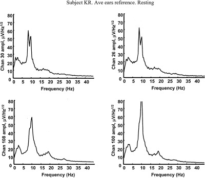
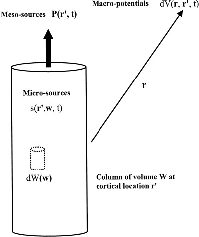
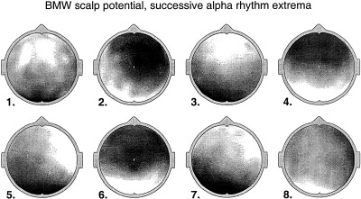
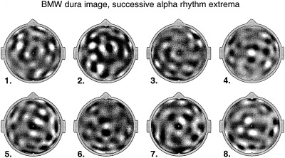
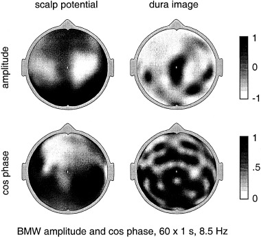
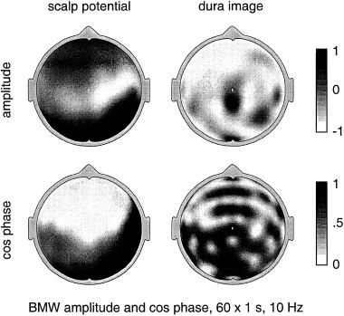
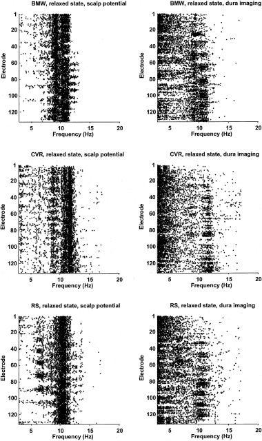
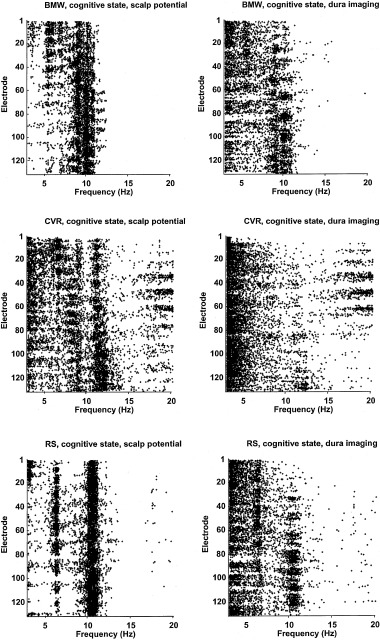
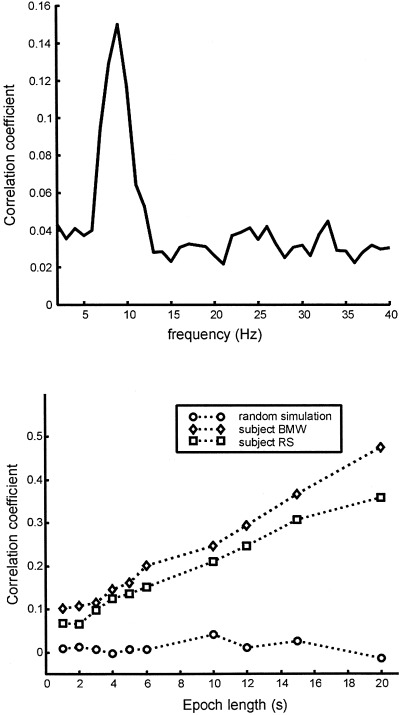
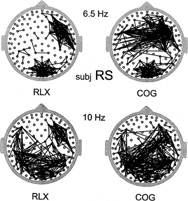
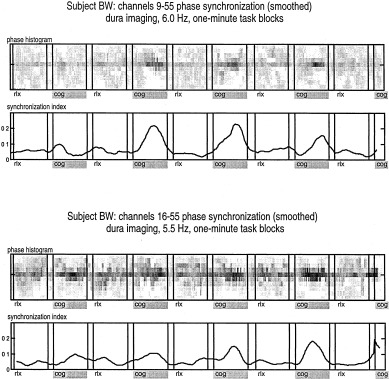
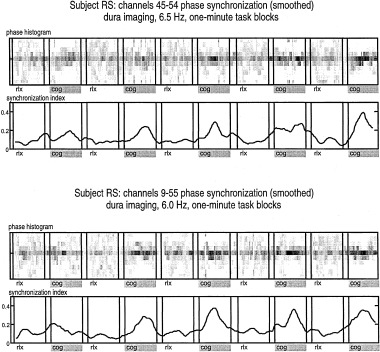
A theoretical framework supporting experimental measures of dynamic properties of human EEG is proposed with emphasis on distinct alpha rhythms. Robust relationships between measured dynamics and cognitive or behavioral conditions are reviewed, and proposed physiological bases for EEG at cellular levels are considered. Classical EEG data are interpreted in the context of a conceptual framework that distinguishes between locally and globally dominated dynamic processes, as estimated with coherence or other measures of phase synchronization. Macroscopic (scalp) potentials generated by cortical current sources are described at three spatial scales, taking advantage of the columnar structure of neocortex. New EEG data demonstrate that both globally coherent and locally dominated behavior can occur within the alpha band, depending on narrow band frequency, spatial measurement scale, and brain state. Quasi-stable alpha phase structures consistent with global standing waves are observed. At the same time, alpha and theta phase locking between cortical regions during mental calculations is demonstrated, consistent with neural network formation. The brain-binding problem is considered in the context of EEG dynamic behavior that generally exhibits both of these local and global aspects. But specific experimental designs and data analysis methods may severely bias physiological interpretations in either local or global directions.

Figure 1

Amplitude spectra based on 5 min of resting EEG (0.2 Hz resolution) with eyes closed, referenced to the (symmetric) digitally averaged potential of the ears. The subject KR is a 38‐year‐old female engineering graduate student. The four locations correspond to left and right frontal and left and right posterior scalp (nose up), roughly sites F3, F4, P3, and P4.

Figure 2

Microcurrent (volume) sources at cell membranes s(r′, w, t) have units microamperes/mm³ and depend on vector location w within cortical column, located at r′, containing elemental volume elements dW(w). The sources are generally the result of synaptic and action potential activity and include (passive) return membrane currents. Microsources generate a dipole moment per unit volume P(r′, t) in each column (or more generally, voxel), depending on source magnitudes and distribution along the column axis. In this multiscale formalism, the intermediate scale dipole moment P(r′, t) can then be identified as the “meso‐source” of the differential scalp potential dV (r, r′, t). Total scalp potential V(r, t) is generally the result of the integrated contribution from all columns (or voxels), located at r′.

Figure 3

The spatial transfer functions 4T_l (potential) and l(l+1)T_l (Laplacian) for a four‐sphere volume conductor model of the head, defined by Eqs (3) and (4). Radial dipole source location is 7.8 cm. Radii of spherical shells are: brain (8.0), CSF (8.2), skull (8.7), and scalp (9.2). Conductivity ratios: brain/CSF (0.2), brain/skull (80.0) and brain/scalp (1.0).

Figure 4

(Upper) A waveform composed of 51 unequally spaced frequency components (roughly 10–175 Hz) with pseudorandom phases simulating an epileptic spike recorded on the dura surface (ECoG). (Lower) The corresponding spatially filtered waveform simulating scalp potential. Obtained from the transfer function T _l and the assumption that temporal frequency is inversely proportional to spatial frequency (as in linear, nondispersive waves). Note scale change. There is no temporal filtering by the volume conductor (consistent with experimental evidence). Rather, the temporal filtering is a byproduct of spatial filtering.

Figure 5

Theoretical estimates of the ratio of dura potential to scalp potential, expressed as a function of “synchronous area” of cortical sources. The three curves were generated by assuming cortical dipole layers of constant (mesoscopic) sources in the head model. The assumed skull‐to‐brain (or scalp) resistivity ratios are shown (40, 80, 120), bracketing the usual estimate of 80. The two triangles are experimental points [Abraham and Ajmone‐Marsan, 1958; Goldensohn, 1979b]. The large arrow near the steep upturn in the curves indicates the clinical observation that epileptic spikes must be synchronous over at least 6 cm² of cortex to be recognized on the scalp [Cooper et al., 1965; Ebersole, 1997].

Figure 6

Theoretical dura electrode sensitivity is plotted as a function of spherical harmonic order l for two electrode diameters, d = 1 and 1.5 cm. Sensitivity (vertical axis) is normalized with respect to its value for a point electrode. Curves are obtained by averaging potentials generated by different spherical harmonic functions (of source distribution, as given by Eq [2]) over the surface area of the electrode.

Figure 7

Simulation study using cortical source distributions at radial location 7.8 cm, each consisting of 3,602 randomly clumped dipole sources. Similar source patterns were used to construct parts 1–3 of Table I. For each source distribution, outer surface potentials were calculated at 131 locations corresponding to electrode positions of EEG experiments. Forward solutions were based on the four‐sphere model used in Figures 3, 4, 5, 6. Inner surface (dura) potentials were estimated with the New Orleans spline‐Laplacian (multiplied by negative sign, lower left) and Melbourne dura image algorithm with zero smoothing parameter (lower right). Point‐by‐point comparisons with actual inner surface potential at 131 dura locations were used to obtain correlation coefficients. Shell radii used by the three‐sphere dura imaging algorithm were 7.9, 8.45, and 9.2 cm, and conductivity ratios were brain/skull (80) and brain/scalp (1). Spline‐Laplacian estimates of dura potential are independent of head model, except for the assumption of a spherical scalp.

Figure 8

Electrode cap with 131 electrodes. The electrode positions were used in both simulations and EEG recordings. The cap was purchased from Electro‐Cap International, Inc.

Figure 9

Amplitude distributions of (average reference) resting alpha rhythm at 8 successive times separated by about 50 ms are shown. The times correspond to alternating positive and negative peaks in the potential recorded by posterior‐midline electrode 130. Each plot was constructed by averaging over five adjacent time slices with 2 ms separation between adjacent slices. Amplitudes were normalized with respect to the maximum positive and negative potentials (yellow and blue, respectively). Subject BMW.

Figure 10

Estimates of dura potential for the same data shown in Figure 9, obtained by passing average reference data through the Melbourne dura imaging algorithm (with smoothing parameter set to zero). Normalized dura potentials are plotted, as in Figure 9. The New Orleans Spline‐Laplacian yields similar patterns of dura potential, e.g., correlation coefficients ≈ 0.95. Addition of uncorrelated 15% noise to the raw data had minimal effect. Subject BMW.

Figure 11

Magnitude (upper row) and cosine phase (lower row) at BMW's lower alpha peak (8.5 Hz) for the average reference potential (left column) and dura image estimate (right column). Plots were obtained by Fourier transforms of 60 successive 1‐sec epochs (1 Hz resolution). Dura image phase plot shows alternating regions at the scale of several centimeters that are 180 degrees out of phase, apparently similar to a wave interference pattern.

Figure 12

Amplitude (upper row) and phase (lower row) at BMW's upper alpha peak (10.0 Hz) for average reference potential (left column) and dura image estimate (right column). Plots were obtained by Fourier transforms of 60 successive 1‐sec epochs (1 Hz resolution). Produced from the same raw data used to produce Figure 11.

Figure 13

Peak power scalp potential (left column) and corresponding dura image (right column) estimates for the three subjects (BMW, CVR, and RS in rows 1–3, respectively). Smaller electrode numbers on vertical axes near the upper parts of plots correspond to more frontal scalp locations (see Fig. 8). For each 5‐sec epoch and each electrode site, the frequency component (0.2 Hz resolution) with the largest power (or amplitude) in the range 3.0 ≤ f ≤ 20.0 Hz was selected by the FFT. Other frequency components at each site are not plotted, even though they may be nearly as large as the peak components. The test was repeated with the same data first passed through the dura image algorithm (right column). Each plot contains 60 epochs × 131 electrodes = 7,860 points. The dominance of alpha band activity over the entire scalp is evident in all three subjects in the average reference potential plots but somewhat less evident in the dura image plots.

Figure 14

Peak power estimates obtained from average reference potentials (left) and dura image estimates (right) for the cognitive periods. Methods are identical to those used in Figure 13, except for some small changes in the number of total epochs.

Figure 15

(Upper) Correlation coefficients comparing successive estimates of cosine dura image phase (over the 131 electrode sites) are plotted vs. integer frequencies. Phase plots were calculated for 5 min of resting alpha using 1‐sec epochs with phase at site 88 (Cz) defined as zero for each epoch. Correlation coefficients were averaged over all 299 successive epoch pairs. Subject BMW. (Lower) Dura cosine phase correlation coefficients comparing successive epochs at individual alpha peaks—10 Hz (subject BMW) and 10 Hz (subject RS) are plotted vs. FFT epoch length. Correlation coefficients, averaged over all epoch pairs, increase monotonically with epoch length, ranging between about 0.1 for 1‐sec epochs to about 0.4–0.5 for 20‐sec epochs (frequency resolution held fixed at 1 Hz). The lower plot (random simulation) was generated using 1/f noise passed through a head model (forward solution) to simulate spatially correlated scalp noise, which was then passed through the dura imaging and FFT algorithms to estimate dura phase.

Figure 16

Dura image interelectrode coherence in the relaxed state for subject RS (RLX, left column, averaged over 5 min) and cognitive state (COG, right column, averaged over 5 min). All interelectrode coherences greater than 0.1 at the 99% confidence level are indicated by lines between the appropriate electrode pair, excluding nearest‐neighbor edge electrodes. Actual coherence estimates vary widely, e.g., from about 0.3 to 0.7 for electrode separations greater than 10 cm. Both upper 6.5 Hz theta coherence (upper row) and 10.0 Hz upper alpha coherence (lower row) generally increased during the cognitive task. However, lower alpha band coherence decreased during the cognitive task (not shown). Simulations confirmed that these patterns represent genuine source coherences rather than volume conduction or statistical artifact.

Figure 17

The upper rows of each plot pair display 10‐sec phase offset distributions (phase differences between electrode pairs) represented as gray‐scale histograms. Successive 1‐min periods of constant brain state are shown, alternating between resting and cognitive states. Cognitive periods are indicated by shaded bars and the word “cog.” The lower row of each plot pair is the synchronization index used by Tass et al. [1998]. Phase offsets peak at approximately 180 degrees. (Upper plot pair) Electrode sites 9–55 (Lower plot pair) sites 16–55 (essentially frontal midline theta). Subject BMW.

Figure 18

Plots similar to Figure 17 for subject RS. (Upper pair) Electrode sites 45–54 (cross‐hemispheric precentral) (Lower pair) sites 9–55. Phase offsets peak at approximately 140 degrees.

References

1. Abeles M (1982): Local cortical circuits. New York: Springer‐Verlag.
1. Abraham K, Ajmone‐Marsan C (1958): Patterns of cortical discharges and their relation to routine scalp electroencephalography. Electroencephalogr Clin Neurophysiol 10: 447–461. - PubMed
1. Andrew C, Pfurtscheller G (1996): Event‐related coherence as a tool for studying dynamic interaction of brain regions. Electroencephalogr Clin Neurophysiol 98: 144–148. - PubMed
1. Andrew C, Pfurtscheller G (1997): On the existence of different alpha band rhythms in the hand area of man. Neurosci Lett 222: 103–106. - PubMed
1. Babiloni F, Babiloni C, Carducci F, Fattorini L, Onorati P, Urbano A (1996): Spline Laplacian estimate of EEG potentials over a realistic magnetic resonance‐constructed scalp surface model. Electroencephalogr Clin Neurophysiol 98: 204–215. - PubMed
Publication types
LinkOut - more resources