A system for the generation of curves on 3D brain images

Abstract

In this study, a computational optimal system for the generation of curves on triangulated surfaces representing 3D brains is described. The algorithm is based on optimally computing geodesics on the triangulated surfaces following Kimmel and Sethian ([1998]: Proc Natl Acad Sci 95:15). The system can be used to compute geodesic curves for accurate distance measurements as well as to detect sulci and gyri. These curves are defined based on local surface curvatures that are computed following a novel approach presented in this study. The corresponding software is available to the research community.

Figure 1

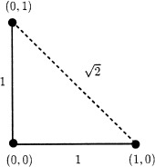
Dijkstra's distance approximation is restricted to travel on graph edges. In this simple example we will get that distance from (1, 0) to (0, 1) is 2, but we know that it is .

Figure 2

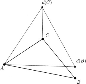
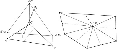
Update procedure for triangle ABC. We want to compute the distance value at C, fitting a plane over the triangle, based on A and B distances, and the desired plane slope g. For simplicity, we assume d(A) = 0.

Figure 3

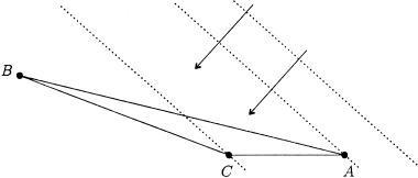
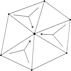
Obtuse triangles in distance computations. Arrows show the growing direction of the distance (i.e., it's negative gradient direction). The front would first reach point A, then C, and finally B. Therefore, C is only supported by A so we can not recover the actual direction of the front. As we restrict the update to come from within the triangle (that is, the gradient direction must lay within the angle equation image, a situation like this can only occur if equation image is obtuse.

Figure 4

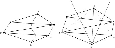
Handling procedure for obtuse triangles. Triangle ABC is divided into two acute triangles, ATC and BTC. Left: Triangulated surface in 3D space. Right: Unfolded surface in the plane. The shaded region shows the limited section of incoming fronts for vertex C.

Figure 5

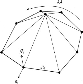
Local neighborhood defined around a given vertex. The contribution of every neighboring triangle must be considered in the distance update procedure.

Figure 6

Building the path using a first order approximation of the distance function. Left: Situation when we are standing over one side of the triangle. Right: If we are standing precisely at a vertex (C), we have one gradient direction (dotted lines) for each neighboring triangle. We choose the one that gives the maximum gradient value in the downward direction.

Figure 7

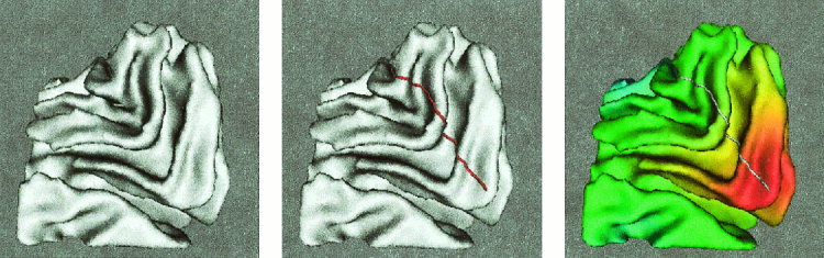
Left: Triangulated data for brain 1. The surface contains 63000 triangles and 31500 points. Center: Geodesic curve obtained with g = 1. Right: Distance values rendered over the surface. Color values range from red (zero distance) to blue (largest distance values).

Figure 8

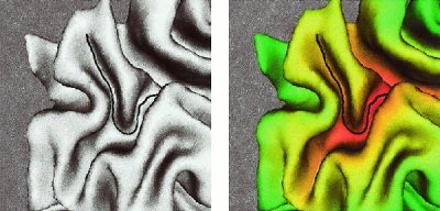
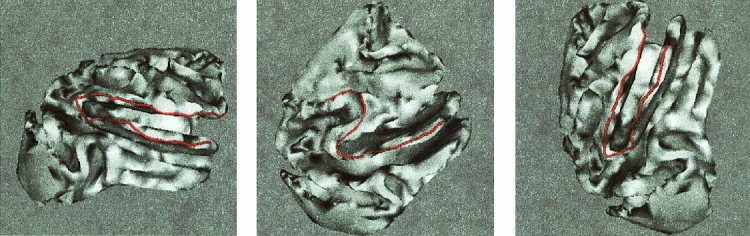
Crease extraction for brain 1. Left: Crease line shown over the original surface. Right: Crease line shown over the curvature‐weighted distance function rendered over the surface.

Figure 9

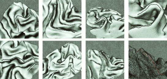
Additional examples of crease extraction for brain 1. The last figure shows the crease line over the triangulated mesh.

Figure 10

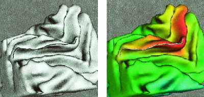
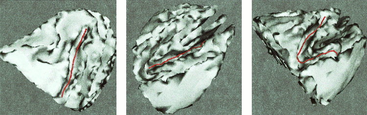
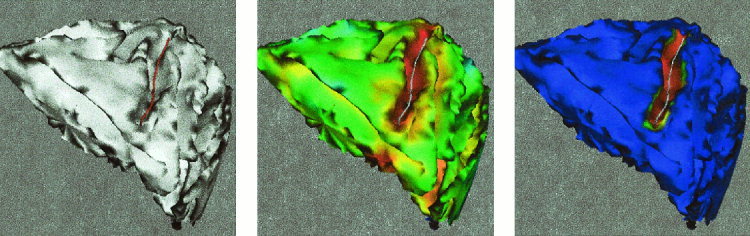
Valley extraction for brain 1. Left: Valley line shown over the original surface. Right: Valley line shown over the curvature‐weighted distance function rendered over the surface. Color reference as before.

Figure 11

Additional examples of valley extraction for brain 1.

Figure 12

Left: Triangulated data for brain 2. The surface contains 7700 triangles and 3800 points. Center: Geodesic curve obtained with g = 1. Right: Distance values rendered over the surface. Color reference as before.

Figure 13

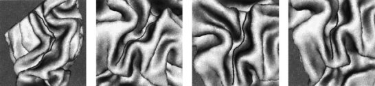
Crease extraction for brain 2.

Figure 14

Valley extraction for brain 2.

Figure 15

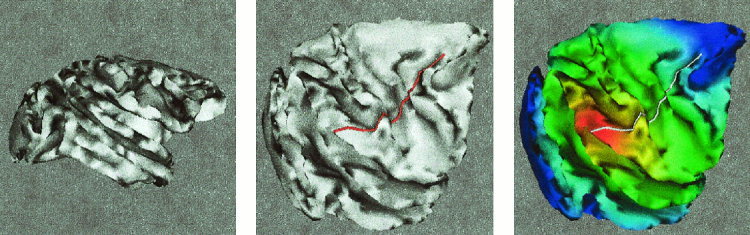
Additional valley extraction example for brain 2. Left: Valley line shown over the original surface. Center: Corresponding weighted distance values are rendered over the surface. Right: The distance function is only computed until we reach the selected end point, thereby further improving the computational time. Color reference as before.

Figure 16

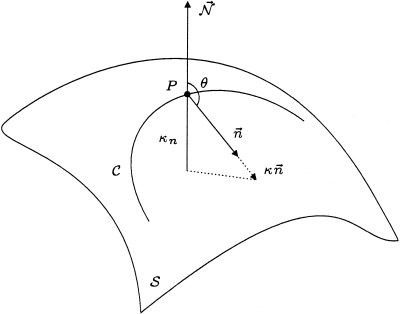
Basic 3D geometry and curvatures.

Figure 17

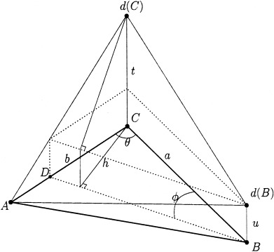
Update procedure for triangle ABC. We want to compute the distance value at C, fitting a plane over the triangle, based on A and B distances, and the desired plane slope g. We require the solution t to be greater than u, and to be updated from within the triangle, that is, h should lay between edges CA and CB.

Figure 18

Undesirable situation caused by splitting obtuse triangles. See text for explanation.

Figure 19

Handling obtuse triangles in the back propagation algorithm. Left: Considering the shown neighborhood leads to the local minima situation. Right: Neighborhood that gives the correct path through the unfolded surface.

Figure 20

Three dimensional view of the triangulated surface element considered to compute the mean curvature using equation (9).

References

-
- Angenent S, Haker S, Tannenbaum A, Kikinis R (1998): Laplace‐Beltrami operator and brain flattening. University of Minnesota ECE Report. - PubMed
- Barth TJ, Sethian JA (1998): Numerical schemes for the Hamilton‐Jacobi and level set equations on triangulated domains. J Comp Physics 145: 1–40.
- Bertalmio M, Sapiro G, Randall G (1999): Region tracking on level‐sets methods. IEEE Trans Med Imaging 18: 448–451. - PubMed
- Bruckstein AM (1988): On shape from shading. Comp Vision Graph Image Process 44: 139–154.
- Caselles V, Kimmel R, Sapiro G, Sbert C (1997): Minimal surfaces based object segmentation. IEEE‐PAMI 19: 394–398.
Publication types
MeSH terms
LinkOut - more resources
Full Text Sources