The cortical representation of the hand in macaque and human area S-I: high resolution optical imaging

Abstract

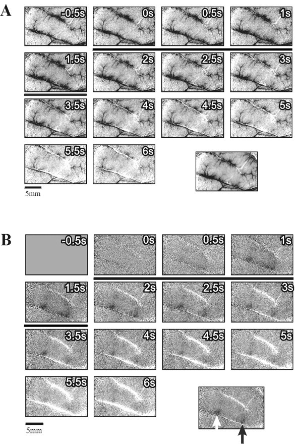
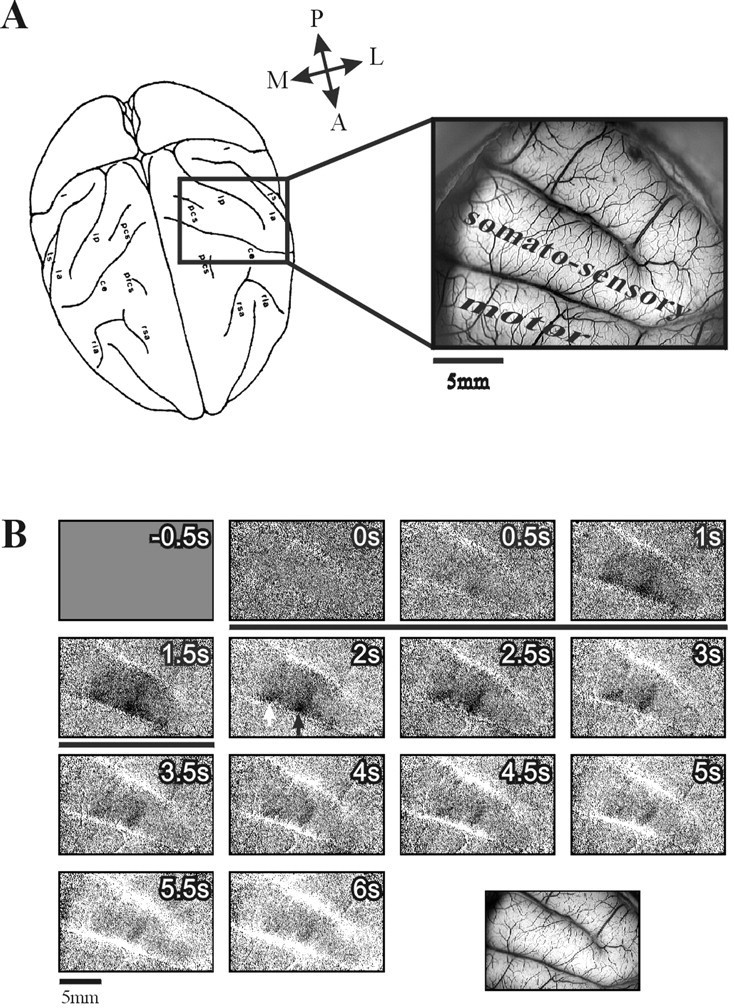
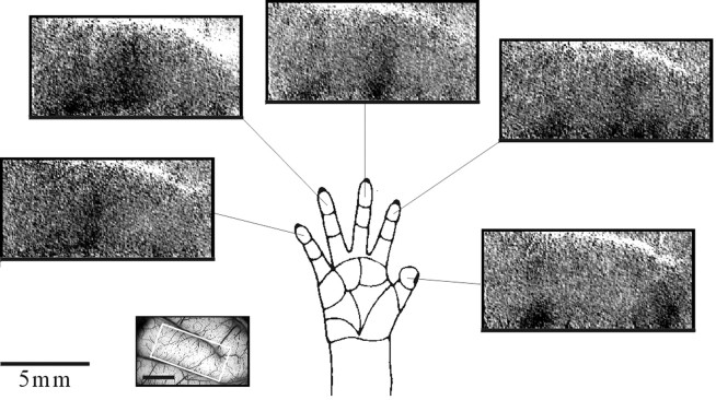
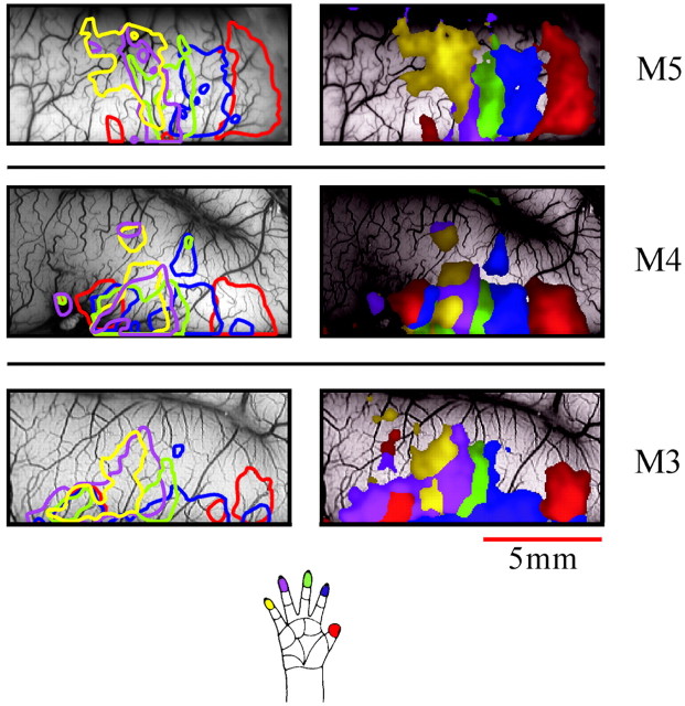
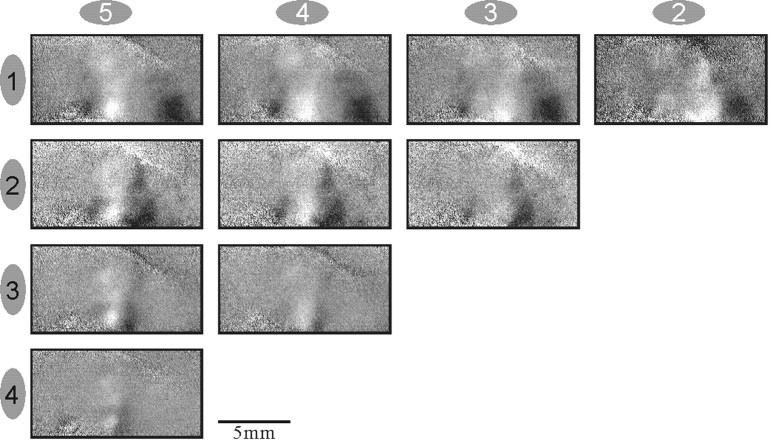
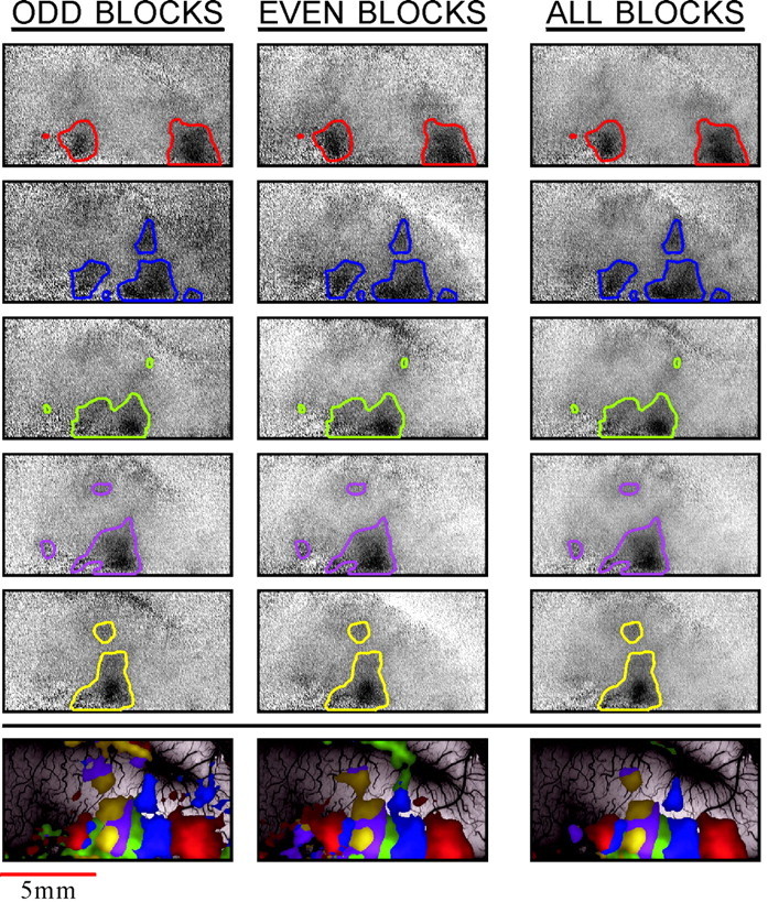
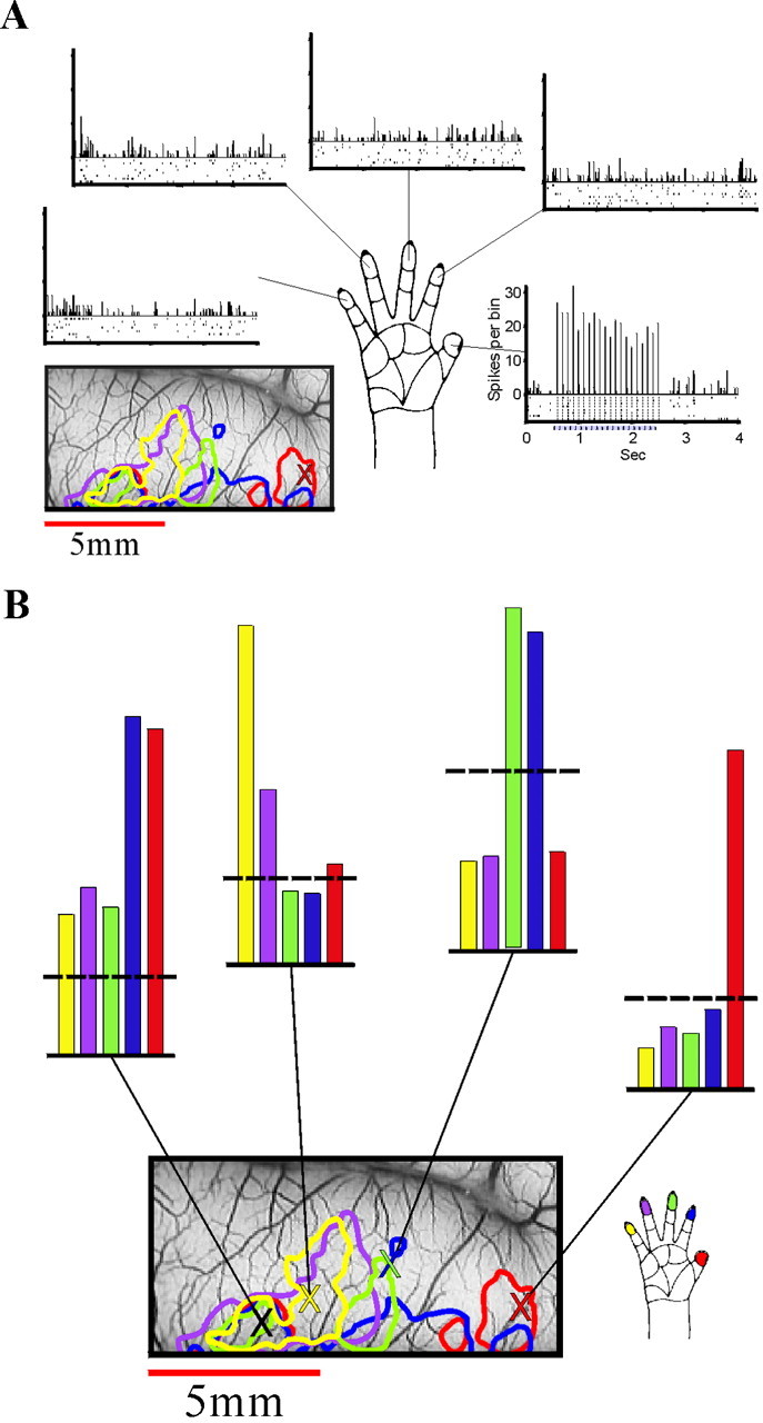
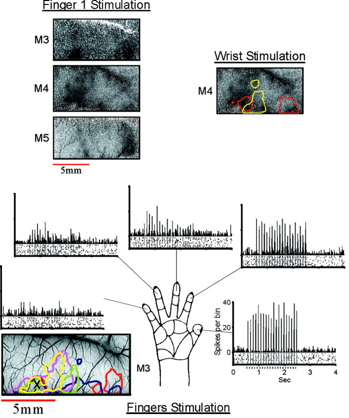
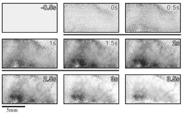
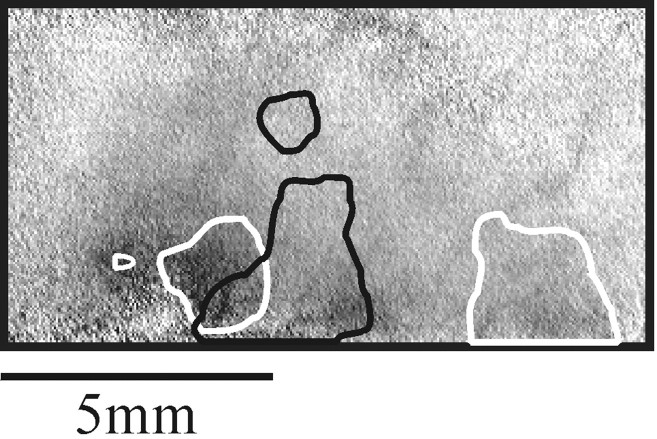
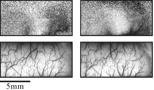
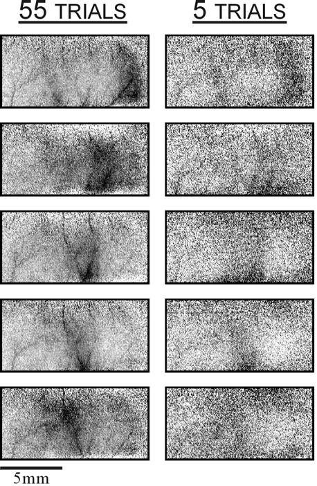
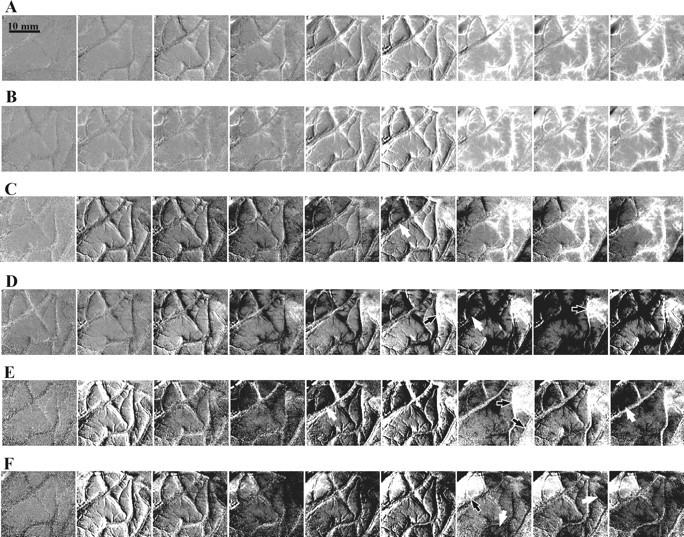
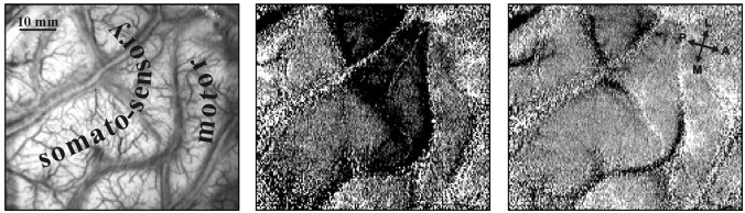
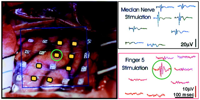
High-resolution images of the somatotopic hand representation in macaque monkey primary somatosensory cortex (area S-I) were obtained by optical imaging based on intrinsic signals. To visualize somatotopic maps, we imaged optical responses to mild tactile stimulation of each individual fingertip. The activation evoked by stimulation of a single finger was strongest in a narrow transverse band ( approximately 1 x 4 mm) across the postcentral gyrus. As expected, a sequential organization of these bands was found. However, a significant overlap, especially for the activated areas of fingers 3-5, was found. Surprisingly, in addition to the finger-specific domains, we found that for each of the fingers, weak stimulation activated also a second "common patch" of cortex, located just medially to the representation of the finger. These results were confirmed by targeted multiunit and single-unit recordings guided by the optical maps. The maps remained very stable over many hours of recording. By optimizing the imaging procedures, we were able to obtain the functional maps extremely rapidly (e.g., the map of five fingers in the macaque monkey could be obtained in as little as 5 min). Furthermore, we describe the intraoperative optical imaging of the hand representation in the human brain during neurosurgery and then discuss the implications of the present results for the spatial resolution accomplishable by other neuroimaging techniques, relying on responses of the microcirculation to sensory-evoked electrical activity. This study demonstrates the feasibility of using high-resolution optical imaging to explore reliably short- and long-term plasticity of cortical representations, as well as for applications in the clinical setting.

Fig. 1.

Improvement of functional maps using first-frame subtraction to remove common slow vascular noise. A, Image sequence obtained with mechanical stimulation of a single fingertip (finger 1) in monkey M3. Each frame was divided by the corresponding frame from the blank condition and scaled such that the full gray scale corresponds to a fractional change of 1.7 × 10⁻³. The specific finger activation is not seen here. Instead, an almost constant noise pattern is evident. This pattern is not related to the stimulus because it appears at the time of the first frame, preceding the stimulus onset (stimulus duration is marked by a black horizontal bar). The image at the bottom right is the average of frames 4–9 (1–4 sec after the stimulus) of the above sequence. Because the dominant noise pattern exists in all of these frames, this averaging does not eliminate it. B, The same image sequence from A after subtracting the average of the first three frames from all subsequent frames. Here the stimulus-evoked activation is evident. Again, the image at the bottom right is the average of frames 4–9 of the above sequence. Thedark patch on the right (black arrow) is the finger 1 domain. The dark patch on the left (white arrow) was activated also with stimulation of other fingers. Further discussion of these activation patterns is given below. The full gray scalein all images corresponds to a fractional change of 1.7 × 10⁻³. s, Seconds.

Fig. 2.

Time course of optical response to mechanical stimulation of a single finger. A, Left, A schematic dorsal view of the macaque brain outlining the cortical territory explored in a typical somatosensory imaging session.Right, Image of the cortical surface (left hemisphere, monkey M3) illuminated with green light (540 nm) to emphasize the blood vessel pattern. The somatosensory and motor areas are marked. The anterior part of the somatosensory strip is Brodmann's area 1, and the posterior part is area 2. B, An image series of the left hemisphere in monkey M3 showing the temporal development of the optical response to a weak mechanical indentation stimulation of finger 3 of the right hand. Each frame represents 500 msec of summation of collected video frames. The image at the bottom rightshows the corresponding vascular image taken with green light (for general orientation, see A). The finger was stimulated at the distal phalanx using the pneumatic stimulator described in the text (Materials and Methods). Air pressure pulses (10 msec) were delivered for 2 sec at a rate of 10 Hz. The stimulus started concurrently with the acquisition of the second frame(stimulus duration is marked by a black horizontal bar). To obtain these images, we divided each image from the sequence obtained during stimulus application by the corresponding image from the blank (no-stimulus) condition. This procedure, in addition to normalizing for the illumination pattern, nearly eliminates the signals coming from respiration and heart pulsation because data acquisition was always synchronized to both of these cycles. First-frame subtraction was applied. Here and in the following figures, activity shows up as darkening in the image. The full gray scale corresponds to a fractional change of 1 × 10⁻³. The images from 45 repetitions of the stimulus (and blank) presentations were averaged. A, Anterior; L, lateral; M, medial;P, posterior.

Fig. 3.

Cortical representation of single fingers. Image sequences like the one in Figure 2B were obtained for stimulation of each of the five fingertips. Frames 4–9 of each series (1–4 sec after the stimulus) were averaged to produce the single-finger activity maps shown here. The resulting images were rotated and cropped to focus on the activated part of the postcentral gyrus. The white rectangle on the vascular imaging at the bottom outlines the cropped area. The maps in all subsequent figures are shown at this orientation. The five images surrounding the hand drawing show the areas activated by mechanical stimulation of the five fingers. A somatotopic organization of the hand representation is evident, with the thumb on the right(anterolateral) and the little finger on the left(posteromedial). In addition to the finger-specific activations, there is a patch of cortex just medial to the hand representation that is activated by all stimuli, including a weak activation by finger 5 (see also Figs. 4, 6, in another monkey). Further discussion of this domain is given below (see Fig. 8). The full gray scalecorresponds to a fractional change of 1 × 10⁻³.

Fig. 4.

Somatotopic organization of the hand area in three monkeys. Left hemisphere finger maps for right-hand stimulation were obtained in a way similar to the way in which the ones in Figure 3 were obtained. The maps from all three monkeys are summarized here in two formats. Left, The images show contour maps from the three monkeys. Contour lines at the level of 30% of peak activation for each finger are superimposed on the surface vasculature image (imaged with green light). Thethin contour lines were computed from a smoothed version of the maps (low-pass filtered with a Gaussian filter, ς = 120 μ). The contour for each finger iscolored according to the color code shown in the hand drawing below the maps. To facilitate a comparison with the second type of analysis shown on the right, the WTA patches are also superimposed. Right, The images show WTA maps calculated from the same data. The information from the individual finger maps is integrated here using a winner-takes-all rule. The color of each pixel is determined by the finger that gave the strongest response, using the same color codes used for the contours. The intensity encodes the amplitude of the response to the “winning” finger. Only pixels in which this response was >30% of the peak activation were colored. The other pixels show the underlying vascular pattern. Also see Figure6.

Fig. 5.

Differential finger maps. The five single-finger maps from monkey M4 were used to generate the differential maps for each pair of fingers. The top row shows the images resulting from subtracting the maps of fingers 2–5 from the finger 1 map; the second row shows the finger 2 map minus the maps of fingers 3–5, and so on. Before the images were subtracted, each map was normalized as explained in Materials and Methods, so that the maximal activation (defined as the minimal value in the smoothed version of the map) was mapped to 1.0 and the median value was mapped to 0.0. Next, the resulting differential maps were all scaled such that the range (−1 to 1) would span the full gray scale.

Fig. 6.

Reproducibility of the finger maps. Theleft and middle columns show two sets of single-finger maps (rows 1–5 from thetop) and WTA maps (bottom row) from independent trials in the same cortex (monkey M4). The finger 1 map is at the top, and the finger 5 map is on row 5. These data were collected in 24 blocks of five trials each. For the reproducibility test, these images were divided into two sets of alternating blocks, and the functional maps were computed separately from each of these sets, containing 12 blocks. The average of the twoleft maps in each row creates the map in theright column. To aid in the comparison, thecontour lines that were computed from the full data set were superimposed on all the maps. The color code is the same as that in Figure 4. The full gray scalecorresponds to a fractional change of 1.2 × 10⁻³.

Fig. 7.

Targeted electrophysiological confirmation of the optical maps. A, The optical maps were used to guide electrode penetrations into optically identified loci. The data in this figure are from a recording in the finger 1 area (as determined by optical imaging) of monkey M3. [The penetration site is marked on the vascular image (bottom left) by a red X.] The contours that summarize the imaging results (see Fig. 4) are also superimposed on the vascular image (below the left spike train). The stimuli used were the same as in the imaging session (at each of the 5 fingertips, 2 sec at 10 Hz). The data recorded from the site representing digit 1 show multiunit responses to stimulation of fingers 1–5 (right toleft, counterclockwise). The spikes collected in eight trials for each stimulus are shown in the raster displays (bottom), and the resulting PSTHs (10 msec bins) are shown on the top. Stimulation of the thumb elicited a strong response with clear entrainment of the spikes to the stimulus pulses (right spike train). Stimulation of the other fingers elicited no response or even slight inhibition (e.g., digits 2–5 particularly during the response onset). The specificity of the response to finger 1 stimulation is very clear, confirming the optical results. B, The multiunit data fromA are summarized here together with data from the three other penetrations, one on the border of digits 2 and 3 (second histogram from the right), one for digit 5, and one from the common patch. The contour finger map from Figure 4 is reproduced here, with marks (X symbols) at the four electrode penetration sites. The tuning curves obtained in each recording site are shown above as color-coded histograms. Thus despite the overlap, the responses are rather tuned. The vertical bars show the normalized spike counts from the 2 sec stimulation period. The dashed horizontal lines show the spontaneous firing level that was computed from the periods with no stimulation. Note that the small inhibition mentioned above is apparent in all three recording sites that correspond to digits 1, 2/3, and 5. Each of the tuning curves was normalized to have a common maximal value.

Fig. 8.

The common patch. Top left, The three images show the cortical activation by stimulation of the thumb in three monkeys. In addition to the finger-specific domain on the lateral (right) side, there is another activated patch on the medial part (left part of the image). This common patch was activated also by stimulation of the other fingers (data not shown). Top right, The map (monkey M4) shows the activity evoked by stimulation of the wrist using the same pneumatic stimulator that was used for the fingers. This activation pattern also includes the common patch. To assist in comparison with the fingers somatotopy, the contour lines of fingers 1–5 from Figure 4 were superimposed on the map. The full gray scale corresponds to a fractional change of 1 × 10⁻³, 1.4 × 10⁻³, and 1.1 × 10⁻³ in the finger 1 images and to 1.1 × 10⁻³ in the wrist image.Bottom, The multiunit data recorded at the common patch of monkey M3 are shown. The format is the same as that used in Figure 7A. The tuning curve is shown in Figure7B.

Fig. 9.

Time course of optical response to electrical stimulation of the median nerve. An image series shows the temporal development of the optical response to a right median nerve stimulation in monkey M4. Each frame represents 500 msec. The median nerve was stimulated at the wrist via a pair of EKG electrodes. Current pulses of 1 msec were delivered for 2 sec at a rate of 10 Hz. The stimulus started concurrently with the acquisition of the secondframe (stimulus duration is marked by a black horizontal bar). The full gray scale corresponds to a fractional change of 1.5 × 10⁻³.

Fig. 10.

Cortical activation by electrical stimulation of the median nerve. An activity map produced by averaging the last six frames from Figure 9 (corresponding to the period 1–4 sec after stimulus onset) is shown. The contour lines of fingers 1 and 5 from Figure 4 are superimposed on the map to aid in comparison with the fingers somatotopy. Note that a much larger area was activated (light gray area darker than the top of the image), but the common patch was the strongest area activated and occupied much of the dynamic range of this figure. Note that median nerve stimulation in different experiments on different monkeys or human subjects often yields highly variable results, presumably because of the difficulty in reproducing exactly the same activation of the nerve in different subjects (data not shown). The full gray scale corresponds to a fractional change of 1.5 × 10⁻³.

Fig. 11.

Stability of cortical maps. Top, The images are differential maps in which the image obtained during simultaneous stimulation of fingers 1 and 2 was divided by the image from stimulation of fingers 3–5. The data for the leftmap were collected at the beginning of the experiment, and the map on the right was obtained ∼28 hr later (in 28 hr, ∼50 different maps can be accumulated under different stimulation conditions). The full gray scale corresponds to a fractional change of 0.8 × 10⁻³(left) and 1.4 × 10⁻³(right). Bottom, The images show the corresponding vascular patterns taken with green light.

Fig. 12.

Rapid functional imaging. Single-finger maps from monkey M5, with finger 1 at the top and finger 5 at thebottom. Right, The images are from a single block of five trials. Left, The corresponding images are averages over 11 such blocks. The data collection for these maps took ∼6 min per block. All images were autoclipped to occupy the full dynamic range of each image.

Fig. 13.

Visualization of spontaneous vascular activity in the human cortex. Each row shows spontaneous changes (without a stimulus) in cortical reflection as a function of time. Frame duration is 500 msec. A, B, Theserows depict an increase in vascular oxygenation level (vessels brighten) over a large cortical area. The full gray scale (clipping range) corresponds to a large fractional change of 2.0 × 10⁻². These two similar events occurred 15 min apart. C, This row shows vascular activation as well as darkening of the parenchyma in a restricted area (white arrow). D–F, These rows depict slow brightening (black arrows) and darkening (white arrows) in a restricted area (clipping range, 2.0 × 10⁻³). To show these small changes, these sequences of cortical images were obtained by subtracting the average of the first three frames in the sequence from each of the cortical images. Images were obtained with 605 nm illumination emphasizing oxygenation changes. Scale bar, 10 mm.

Fig. 14.

Intraoperative imaging of the somatosensory hand area using median nerve stimulation. Left, Image of the cortical surface (left hemisphere) illuminated with green light (540 nm) to emphasize the blood vessel pattern. The somatosensory and motor stripes as determined by optical imaging and confirmed with an electrocorticogram (see Fig. 15) are marked. Middle, Optical map of the area activated by median nerve stimulation. To minimize the noise, trials showing large vascular noise (such as that seen in Fig. 13A,B) above a fixed preset value were autorejected by the analysis program. To obtain this functional map, the average image (16 trials) from the stimulated conditions was divided by the average image from the blank condition (no stimulus, 16 trials). Right, Flat map showing the control map obtained by dividing the sum of the same blank condition by another independent set of the second blank condition we used as a control (16 trials each).

Fig. 15.

Electrocorticographic confirmation of the optical map. Left, A photographic image of the exposed cortex with the array of surface electrodes (4 × 5) that were used to record somatosensory-evoked potentials (boxed area).Right, Electrical traces showing the evoked potentials that were recorded simultaneously from eight electrodes (coloredyellow on the photo). The arrangement of the traces mirrors the position of the corresponding electrodes (see Materials and Methods). The top set of traces (blue) shows responses to electrical stimulation of the median nerve, and thebottom traces (red) show the response to tactile stimulation to the tip of finger 5. Each trace is actually a composite, consisting of two superimposed traces representing the average from two independent sets of trials (128 repetitions for the median nerve and 256 repetitions for the finger 5 stimulation).

References

1. Bakin JS, Kwon MC, Masino SA, Weinberger NM, Frostig RD. Suprathreshold auditory cortex activation visualized by intrinsic signal optical imaging. Cereb Cortex. 1996;6:120–130. - PubMed
1. Bonhoeffer T, Grinvald A. The layout of iso-orientation domains in area 18 of cat visual cortex: optical imaging reveals a pinwheel-like organization. J Neurosci. 1993;13:4157–4180. - PMC - PubMed
1. Bonhoeffer T, Kim DS, Malonek D, Shoham D, Grinvald A. Optical imaging of the layout of functional domains in area 17 and across the area 17/18 border in cat visual cortex. Eur J Neurosci. 1995;7:1973–1988. - PubMed
1. Buonomano DV, Merzenich MM. Cortical plasticity: from synapses to maps. Annu Rev Neurosci. 1998;21:149–186. - PubMed
1. Cannestra AF, Black KL, Martin NA, Cloughesy T, Burton JS, Rubinstein E, Woods RP, Toga AW. Topographical and temporal specificity of human intraoperative optical intrinsic signals. NeuroReport. 1998;9:2557–2563. - PubMed
Publication types