Neural coding mechanisms underlying perceived roughness of finely textured surfaces

Abstract

Combined psychophysical and neurophysiological studies have shown that the perceived roughness of surfaces with element spacings of >1 mm is based on spatial variation in the firing rates of slowly adapting type 1 (SA1) afferents (mean absolute difference in firing rates between SA1 afferents with receptive fields separated by approximately 2 mm). The question addressed here is whether this mechanism accounts for the perceived roughness of surfaces with element spacings of <1 mm. Twenty triangular and trapezoidal gratings plus a smooth surface were used as stimulus patterns [spatial periods, 0.1-2.0 mm; groove widths (GWs), 0.1-2.0 mm; and ridge widths (RWs), 0-1.0 mm]. In the human psychophysical studies, we found that the following equation described the mean roughness magnitude estimates of the subjects accurately (0.99 correlation): 0.2 + 1.6GW - 0.5RW - 0.25GW(2). In the neurophysiological studies, these surfaces were scanned across the receptive fields of SA1, rapidly adapting, and Pacinian (PC) afferents, innervating the glabrous skin of anesthetized macaque monkeys. SA1 spatial variation was highly correlated (0.97) with human roughness judgments. There was no consistent relationship between PC responses and roughness judgments; PC afferents responded strongly and almost equally to all of the patterns. Spatial variation in SA1 firing rates is the only neural code that accounts for the perceived roughness of surfaces with finely and coarsely spaced elements. When surface elements are widely spaced, the spatial variation in firing rates is determined primarily by the surface pattern; when the elements are finely spaced, the variation in firing rates between SA1 afferents is determined by stochastic variation in spike rates.

Fig. 1.

Stimulus patterns. A, Drum with grating stimuli machined into its surface and photographs of typical monkey and human distal fingerpads. Note the differences in skin ridge patterns between humans and monkeys. B, Cross-sectional view of a trapezoidal (left) and triangular (right) grating. C, Groove and ridge widths of all 21 gratings. The surfaces were designed so that almost all spatial periods (except 0.1 mm) comprised two or more combinations of GW and RW (dashed lines), almost all GWs (except 0.3 mm) were paired with two or more RWs (solid lines), and most RWs were paired with two or more GWs. The surface at 0 mm GW and RW is the smooth surface.

Fig. 2.

Psychophysical roughness judgments versus groove and ridge width. The y-axis in each graph represents the mean normalized roughness judgments from 10 subjects (SEM averaged 0.063; range, 0.013–0.125). The lines in each graph represent the values predicted by the following equation: 0.2 + 1.6GW − 0.5RW − 0.25GW².A, Roughness judgments are separated into three groups on the basis of RW to show the correspondence with the equation evaluated at three values of RW (0, 0.5, and 1.0 mm). B,Symbols of a single type represent roughness judgments at single GW values (in millimeters). C, Thex-axis represents the best (least squares) fitting equation involving all linear and second-order terms in GW and RW that are statistically significant.

Fig. 3.

Raster plots of SA1, RA, and PC responses to gratings. Each tick mark represents the occurrence of an action potential, and each horizontal row ofticks represents the response to a single sweep of the stimulus pattern across the receptive field at a velocity of 20 mm/sec.Successive rows represent response sweeps of action potentials after consecutive 200 μm shifts of the stimulus perpendicular to the scanning direction. The rasters in a single column represent responses to a surface with a single spatial period, which is specified at the bottom. The grating with the 0.1 mm spatial period is a triangular grating. The rest are trapezoidal gratings with groove widths that are as close to half of the spatial period as the design allows (0.1, 0.2, 0.3, 0.4, 0.6, 1.0, and 1.0 mm groove widths for the 0.2, 0.4, 0.6, 0.8, 1.0, 1.5, and 2.0 mm spatial periods, respectively).

Fig. 4.

Summed cycle histograms of responses to fine gratings. The spatial period (SP) and ridge width of each column of histograms (A–E) are shown in the top right corner of thetop histogram. Histograms of individual neuronal responses to each grating were rotated to center the peak response and then summed across neurons to produce the histograms displayed here (see Materials and Methods).

Fig. 5.

Strength of entrainment to the grating spatial period. Vector strength represents the degree to which impulse firing is entrained by the grating cycles. A value of one corresponds to firing that occurs at only one phase location relative to the passing grating cycles; a value of zero corresponds to uniform firing across all phase locations. Each filled circle represents the vector strength of a composite cycle histogram, five of which are displayed for each afferent type in Figure 4. The filled triangles represent the vector strengths expected by chance if there was no cyclic entrainment; the error bars represent the 95% confidence intervals (i.e., the region within which vector strength would fall 95% of the time if there was no cyclic entrainment; see Materials and Methods).

Fig. 6.

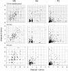
Serial interspike intervals for SA1, RA, and PC responses. Intervals 1 and 2 represent successive intervals within a single sweep. Each plot represents all serial interval pairs evoked by the specified grating for all sweeps and all neurons of the specified type. The units are millimeters. The grid lines represent multiples of a single grating cycle.Points close to the grid lines represent intervals that were close to a multiple of the grating cycle.

Fig. 7.

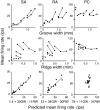
SA1, RA, and PC mean impulse rates versus groove width, ridge width, and the predicted impulse rates. Solid lines in the toptwo rows linkpoints with the same spatial period. For example, thethree points linked by a line in each of these graphs are impulse rates evoked by gratings with 2 mm spatial periods. The solid lines in the bottom row are the predicted impulse rates. Ther² values are 0.97, 0.81, and 0.16 for the SA1, RA, and PC regressions, respectively. The PC regression is not significant. ips, Impulses per second.

Fig. 8.

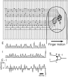
Spatial variation calculations. The model illustrated here corresponds to the calculations used to compute the spatial variation in SA1 firing rates. The hypothesis is that roughness perception is the rectified differences in firing rates between skin regions with centers separated by 1–3 mm. A neuron withE and I subfields like those illustrated here and with an impulse rate that is proportional to the difference between the E and I drive at any instant computes the parameter expressed by the spatial variation hypothesis. The diagram illustrates a finger scanning from left toright across a grating with 0.2 mm groove and ridge widths (0.4 mm spatial period). The finger and grating are not drawn to the same scale. The E and I regions represent hypothetical excitatory and inhibitory areas, each receiving inputs from six SA1 afferents as an example. The actual number varies from 2 to 20 in the computations. The individual spike trains displayed here were drawn at random from the whole set of responses to the grating with 0.2 mm groove and ridge widths. Theverticalgray bars in therows marked E and Irepresent the summed impulses in 12.5 msec bins in the excitatory and inhibitory afferents, respectively. The solid linerepresents a smoothed (Gaussian kernel, 5 msec SD) estimate of the instantaneous rate. The row marked E–Iplots the difference between E and Iexpressed as summed impulse rates. It is meant to represent the net excitatory drive that, when positive, produces a mean firing rate proportional to the difference in firing rates between afferents from the E and I subfields.

Fig. 9.

Consistency plot of perceived roughness versus spatial variation of SA1 neural firing rates. Spatial variation was computed with an algorithm that is illustrated in Figure 8 (see Results). Correlation, 0.97.

Fig. 10.

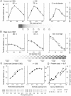
Perceived roughness and measures of spatial variation in firing rates in four studies with different textured surfaces. The lefty-axis in each graph is the mean reported roughness. The righty-axis is the spatial variation in SA1 firing rates. The surface pattern used in each study is illustrated below the data to which the pattern applies. The impulse rates from the first three studies have been rescaled to be approximately consistent with the rates in the present study. A, Results from Connor et al. (1990) who used 18 raised-dot patterns with different mean dot spacings and diameters. The pattern segment corresponding to each dot spacing is shown below the data. B, Results from Blake et al. (1997) who used 18 raised-dot patterns with different dot heights and diameters. The pattern segment corresponding to each mean dot diameter is shown below the data. C, Results fromConnor and Johnson (1992) who varied pattern geometry to distinguish temporal and spatial neural coding mechanisms. D, Data from the present study. The solid lines connect stimulus patterns with constant spatial periods as in Figure 7.

References

1. Blake DT, Hsiao SS, Johnson KO. Neural coding mechanisms in tactile pattern recognition: the relative contributions of slowly and rapidly adapting mechanoreceptors to perceived roughness. J Neurosci. 1997;17:7480–7489. - PMC - PubMed
1. Connor CE, Johnson KO. Neural coding of tactile texture: comparisons of spatial and temporal mechanisms for roughness perception. J Neurosci. 1992;12:3414–3426. - PMC - PubMed
1. Connor CE, Hsiao SS, Phillips JR, Johnson KO. Tactile roughness: neural codes that account for psychophysical magnitude estimates. J Neurosci. 1990;10:3823–3836. - PMC - PubMed
1. Cox DR, Lewis PAW. The statistical analysis of series of events. Methuen; London: 1966.
1. Craig JC, Johnson KO. The two-point threshold: not a measure of tactile spatial resolution. Curr Dir Psychol Sci. 2000;9:29–32.
Publication types
LinkOut - more resources