An analysis of neural receptive field plasticity by point process adaptive filtering

Abstract

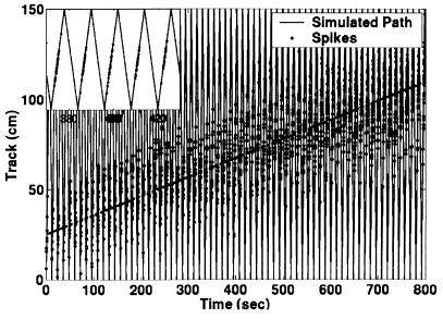
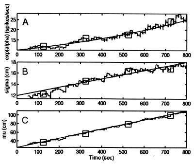
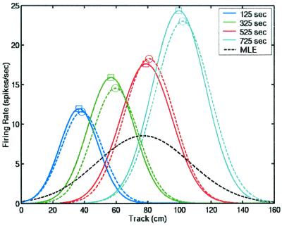
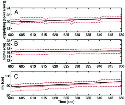
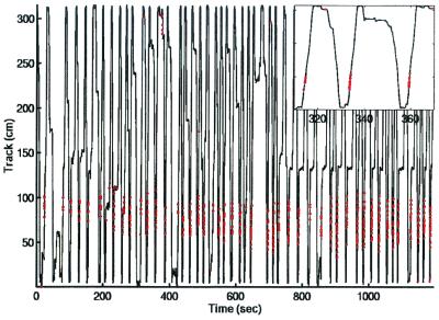
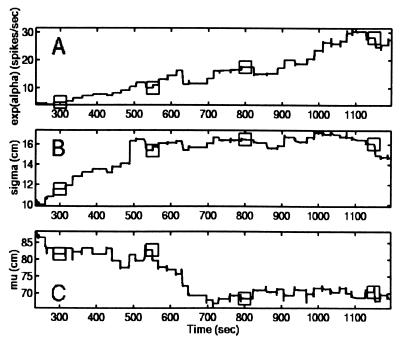
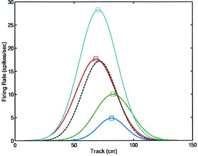
Neural receptive fields are plastic: with experience, neurons in many brain regions change their spiking responses to relevant stimuli. Analysis of receptive field plasticity from experimental measurements is crucial for understanding how neural systems adapt their representations of relevant biological information. Current analysis methods using histogram estimates of spike rate functions in nonoverlapping temporal windows do not track the evolution of receptive field plasticity on a fine time scale. Adaptive signal processing is an established engineering paradigm for estimating time-varying system parameters from experimental measurements. We present an adaptive filter algorithm for tracking neural receptive field plasticity based on point process models of spike train activity. We derive an instantaneous steepest descent algorithm by using as the criterion function the instantaneous log likelihood of a point process spike train model. We apply the point process adaptive filter algorithm in a study of spatial (place) receptive field properties of simulated and actual spike train data from rat CA1 hippocampal neurons. A stability analysis of the algorithm is sketched in the. The adaptive algorithm can update the place field parameter estimates on a millisecond time scale. It reliably tracked the migration, changes in scale, and changes in maximum firing rate characteristic of hippocampal place fields in a rat running on a linear track. Point process adaptive filtering offers an analytic method for studying the dynamics of neural receptive fields.

Figure 1

Simulated dynamics of a single place cell's spiking activity recorded from a rat running back and forth on a 150-cm linear track at a constant speed of 25 cm/sec for 800 sec. The vertical axis is space, and the horizontal axis is time. The vertical lines show the animal's path, and the dots indicate the location of the animal when the neuron discharged a spike. The spiking activity is unidirectional; the cell fires only when the animal moves from the top to the bottom of the track, as seen in the Inset. Simulations used an inhomogeneous Poisson model for Eq. 3.1. Over the 800 sec, the place field parameters evolved as follows: exp(α), the maximum spike rate grew from 10 to 25 spikes per sec; σ, the place field scale, expanded from 12 to 18 cm; and μ, the place field center, migrated from 25 to 125 cm. The solid diagonal line is the true trajectory of μ.

Figure 2

True parameter trajectories and the adaptive estimates of parameter trajectories for the place field model in Eq. 3.1. The straight (wavy) line is (A). True (estimated) trajectory of the maximum spike rate, exp(α). (B) True (estimated) trajectory of the scale parameter, σ. (C) True (estimated) trajectory of the place field center, μ. Adaptive estimates were updated every 1 msec. Squares on the estimated parameter trajectories at 125, 325, 525, and 725 sec indicate the times at which the place fields in Fig. 3 are evaluated. The algorithm accurately tracked the temporal evolution of the model parameters.

Figure 3

Evolution of the true (dashed lines) and adaptive estimates (solid lines) of the place fields. The place fields are shown at 125 (blue), 325 (green), 525 (red), and 725 (aqua) sec. The black dashed line is the ML estimate of the place field based on all the spikes in the 800 sec. By ignoring the temporal evolution of the place field, the ML estimate gives a misleading description of the field's true characteristics, representing it incorrectly as a low-amplitude broad structure that spans the entire track.

Figure 4

Simulation study of the adaptive filter algorithm (Eq. 3.3) by using 50 realizations of the place cell model in Eq. 3.1 and the parameters in Fig. 1. Only 50 sec of the full trajectories are displayed with expanded scales to aid visualization. The true trajectory (black solid line) is shown along with the average of the adaptive estimates of the trajectory (red solid line). Approximate 95% confidence bounds (red dashed lines) were computed for each parameter. (A) exp(α); (B) σ; and (C) μ. All true trajectories are within the 95% confidence bounds, and all estimated trajectories are close to the true trajectories.

Figure 5

Place-specific firing dynamics of an actual CA1 place cell recorded from a rat running back and forth on a 300-cm U-shaped track for 1,200 sec. The track was linearized to display the entire experiment in a single graph. The vertical lines show the animal's position, and the red dots indicate the times at which a spike was recorded. The Inset is an enlargement of the display from 320 to 360 sec to show the cell's unidirectional firing, i.e., spiking only when the animal runs from the bottom to the top of the track.

Figure 6

Adaptive filter estimates of the trajectories. (A) Maximum spike rate, exp(α); (B) place field scale, σ; and (C) place field center μ. Adaptive estimates were updated at 1-msec intervals. The squares at 300, 550, 800, and 1,150 sec are the times at which the place fields are displayed in Fig. 7. The growth of the maximum spike rate (A), the variability of the place field scale (B), and the migration of the place field center (C) are all readily visible.

Figure 7

Estimated place fields at times 300 (blue), 550 (green), 800 (red), and 1,150 (aqua) sec. As in Fig. 3, the black dashed line is the ML estimate of the place field obtained by using all the spikes in the experiment. The ML estimate ignores the temporal evolution of the place field (see Fig. 3).

References

1. Donoghue J P. Curr Opin Neurobiol. 1995;5:749–754. - PubMed
1. Weinberger N M. Curr Opin Neurobiol. 1993;3:570–577. - PubMed
1. Pettet M W, Gilbert C D. Proc Natl Acad Sci USA. 1992;89:8366–8370. - PMC - PubMed
1. Jog M S, Kubota Y, Connolly C I, Hillegaart V, Graybiel A M. Science. 1999;286:1745–1749. - PubMed
1. Mehta M R, Barnes C A, McNaughton B L. Proc Natl Acad Sci USA. 1997;94:8918–8921. - PMC - PubMed
Publication types
LinkOut - more resources