Bayesian haplotype inference for multiple linked single-nucleotide polymorphisms

Abstract

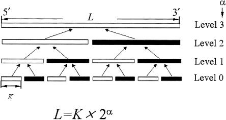
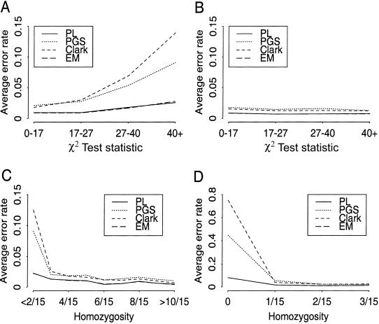
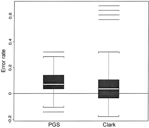
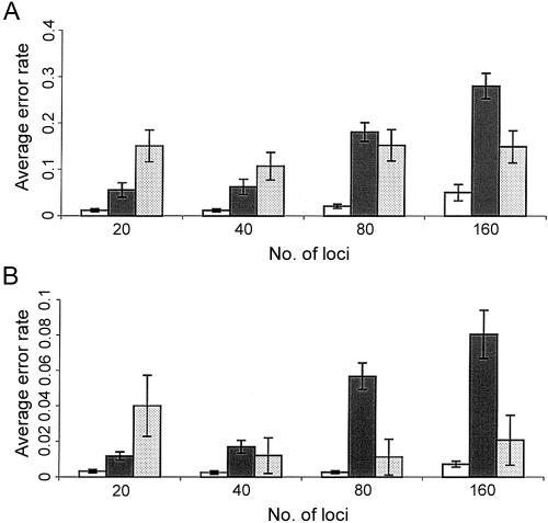
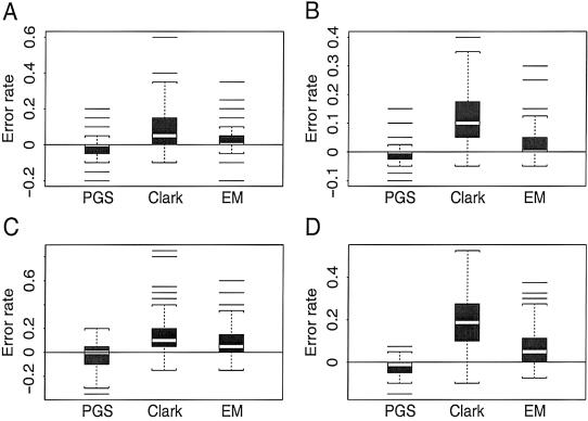
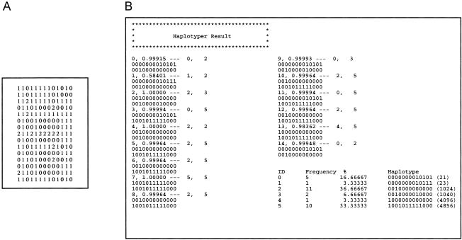
Haplotypes have gained increasing attention in the mapping of complex-disease genes, because of the abundance of single-nucleotide polymorphisms (SNPs) and the limited power of conventional single-locus analyses. It has been shown that haplotype-inference methods such as Clark's algorithm, the expectation-maximization algorithm, and a coalescence-based iterative-sampling algorithm are fairly effective and economical alternatives to molecular-haplotyping methods. To contend with some weaknesses of the existing algorithms, we propose a new Monte Carlo approach. In particular, we first partition the whole haplotype into smaller segments. Then, we use the Gibbs sampler both to construct the partial haplotypes of each segment and to assemble all the segments together. Our algorithm can accurately and rapidly infer haplotypes for a large number of linked SNPs. By using a wide variety of real and simulated data sets, we demonstrate the advantages of our Bayesian algorithm, and we show that it is robust to the violation of Hardy-Weinberg equilibrium, to the presence of missing data, and to occurrences of recombination hotspots.

Figure 1

A schematic depicting the PL algorithm. L denotes the total number of loci; K denotes the number of loci in the smallest segment; α is the highest level of the PL pyramidal hierarchy.

Figure 2

The impact that HWE violation has on the performances of the PL algorithm, the PGS algorithm, Clark's algorithm, and the EM algorithm. The simulation study was conducted under five scenarios, each with 1,000 replications: (1) neutral, (2) moderate heterozygosity, (3) strong heterozygosity, (4) moderate homozygosity, and (5) strong homozygosity. For each trial, a χ² test statistic for testing HWE (after pooling the categories with small counts, this gives rise to the independence test of a 4×4 table, which has 9 df) was computed, the number of homozygotes was counted, and the error rates of each algorithm were recorded. A, Average error rate (defined as the number of erroneous phase calls divided by the total number of phase calls) of each method versus HWE χ² test statistic after combining simulations from models (1), (2), and (3). B, Average error rate versus HWE χ² test statistic after combining simulations from models (1), (4), and (5). Note that the χ² values of 21.67, 16.92, and 14.68 correspond to the 99th, 95th, and 90th percentiles, respectively. C, Average error rate versus sample haplotype homozygosity after combining all simulations. D, Zoom-in view of panel C at left tail of the homozygosity distribution (i.e., 0/15–3/15).

Figure 3

Box plots of δ_A=E_A-E_PL, where E_A and E_PL denote numbers of erroneous phase calls made by algorithm A (the PGS algorithm or Clark’s algorithm) and the PL algorithm, respectively, in each data set. The higher the value the worse algorithm A is in comparison to the PL algorithm. One hundred data sets were simulated; each set consisted of 28 hypothetical individuals whose genotypes were generated by randomly permuting 56 of the 57 complete haplotypes of the 23 linked SNPs near the CFTR gene provided by Kerem et al. (1989).

Figure 4

Histograms of average error rates (number of erroneous phase calls divided by the total number of phase calls) for simulations based on the bottleneck model. We generated 100 independent data sets, each of which consisted of n pairs of unphased chromosomes with L linked SNPs. The chromosomes in each data set are drawn randomly from a simulated population of the 102d-generation descendants of a founder group of 30 ancestors (with mutation rate 10^-5 and crossover rate 10^-3 per generation). The growth rate for the first two generations was 2.0, and that for the remaining generations was 1.05. The error bars are shown as ±1 standard error. The error rates of the PL algorithm (open bars), of the PGS algorithm (shaded bars), and of Clark’s algorithm (dotted bars), for L=20, 40, 80, 160 and for n=20 (A) and n=40 (B), respectively.

Figure 5

Box plots of δ_A=E_A-E_PL, where E_A and E_PL refer to the numbers of erroneous phase calls made by algorithm A (the PGS algorithm, Clark’s algorithm, or the EM algorithm) and the PL algorithm, respectively, for each simulated data set. All the simulated data sets were based on the coalescence model and were obtained from the Simulation Gametes program of the Long Lab. A total of 100 replications were performed for a regional size of 10 units of 4Nc, each of which consisted of n pairs of unphased chromosomes with L linked SNP loci. A, L=8, and n=20. B, L=8, and n=40. C, L=16, and n=20. D, L=16, and n=40.

Figure A1

A, Input file format for HAPLOTYPER. Each line in the input file represents the marker data for each subject; in each line, each SNP occupies one space, and no white spaces are allowed between the neighboring loci. For each SNP, “0” denotes heterozygote, “1” denotes homozygous wild type, “2” denotes homozygous mutant, “3” denotes that both alleles were missing, “4” denotes that only the wild-type allele—“(A,*)”—was known (in the notation, “A” denotes the wild-type allele, and “*” denotes the unknown allele), and “5” denotes that only the mutant allele was known. B, Output file format for HAPLOTYPER. The output file consists of two parts: The first part lists the two predicted haplotypes with their individual identification designations and the associated posterior probabilities. The second part is the summary of the overall haplotype frequency estimated from this sample. If the number of SNPs is >20, we also included a haplotype code (shown in parentheses), which is a decimal number converted from the binary sequence of the haplotype configuration (e.g., haplotype 101 is converted to 2²+2⁰=5).