Nonlinear phase desynchronization in human electroencephalographic data

Abstract

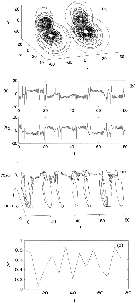
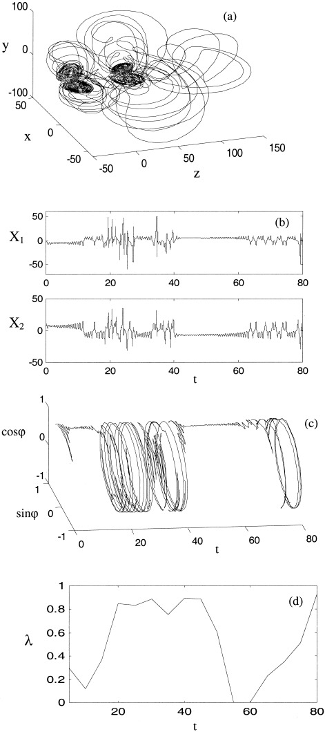
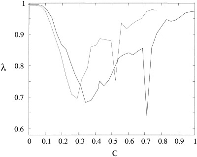
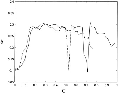
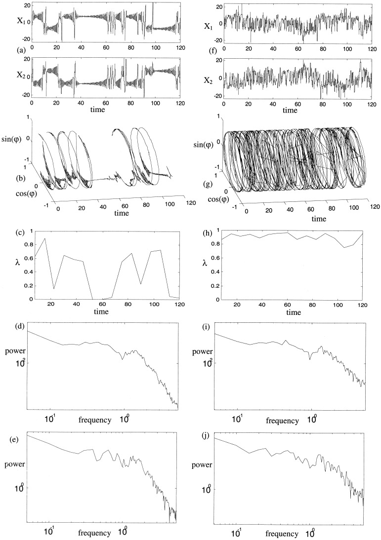
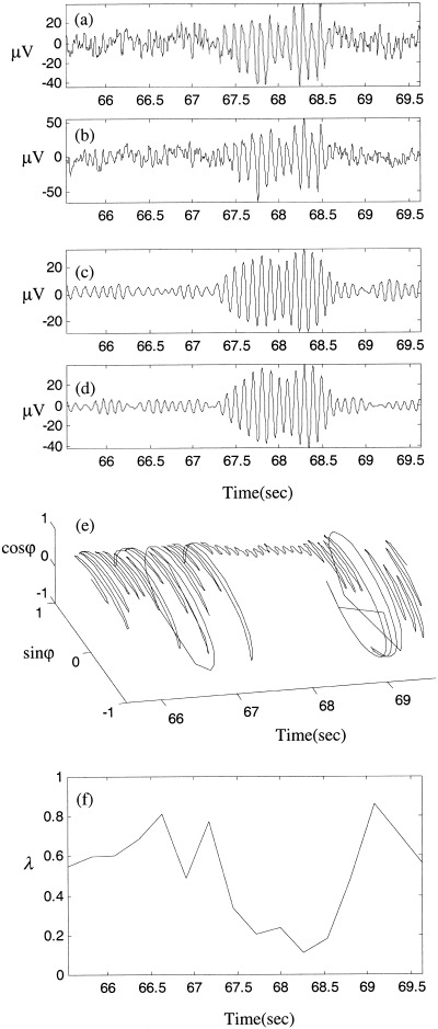
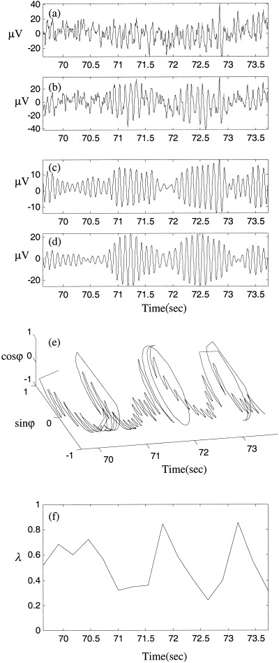
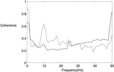
Ensembles of coupled nonlinear systems represent natural candidates for the modeling of brain dynamics. The objective of this study is to examine the complex signal produced by coupled chaotic attractors, to discuss their potential relevance to distributed processes in the brain, and to illustrate a method of detecting their contribution to human EEG morphology. Two measures of quantifying the behavior of coupled nonlinear systems are presented: a measure of phase synchrony and a novel measure of intermittent phase desynchronization. These are used to quantify the behavior of numerical examples of coupled chaotic attractors. Experimental evidence of their contribution to the morphology of the human alpha rhythm is then illustrated in a study of EEG recordings from 40 healthy human subjects. Amplitude-adjusted phase-randomized surrogate data is used to test the null hypothesis that the observed patterns of phase coherence can be described by purely linear methods. Statistical analysis reveals that this null hypothesis can be robustly rejected in a small number (approximately 4%) of EEG epochs. These findings are discussed with reference to the adaptive function and complex dynamics of the brain.

Figure 1

Phase entropy, λ vs. N = number of partitions in equations (7) and (8).

Figure 2

Orbits on the Lorenz attractor and the three hyperbolic fixed points. Two unstable spiral points (dots) each with a single attracting inset (W′ _s and W″ _s) are separated by an unstable saddle point at the origin (diamond) with a stable planar inset (W _s × 2) and single repelling outset (W _u). Axes are the dependant variables in equation (13) with C = 0.

Figure 3

Timeseries and phase entropy for linearly coupled Lorenz systems (equation 13) for coupling strength C = 0.13. (a) Coupled chaotic attractors, with second attractor offset to the right for graphical clarity. (b) Chaotic timeseries for x ₁ (top) and x ₂ (lower). (c) Temporal evolution of the phase difference with axes of sinϕ, cosϕ and time. (d) Temporal evolution of the phase entropy, with timeseries divided into 16 subintervals. (e) Phase entropy as a function of linear coupling strength.

Figure 4

Exemplar synchronous epoch between coupled Lorenz systems (equation 14) with weak nonlinear coupling, C = 0.1. Axes and panels are as for Figure 3a–d.

Figure 5

With moderate nonlinear coupling (C = 0.4) high amplitude excursions appear, corresponding to desynchronous bursts. A this point, phase entropy has approached its global minimum (λ = 0.6) for these non‐linearly coupled systems (equation 14). Axes and panels are as for Figure 3a–d.

Figure 6

With strong nonlinear coupling the desynchronous excursions are increasingly long and disorganized. Axes and panels are as for Figure 3a–d. This example is with asymmetric coupling, C = 0.6.

Figure 7

The relationship between phase entropy and coupling strength for the coupled Lorenz systems with nonlinear, symmetrical coupling (solid) and non‐linear asymmetric coupling (dot‐dot). Results are the average of 20 runs at each coupling strength with t = 160′ and exclusion of an initial transient of t = 160′.

Figure 8

Shannon entropy irregularity δ versus nonlinear coupling strength for the systems (equation 14) and (equation 15). Irregularity here is measured for 32 subdivisions across a timescale of 160′ after exclusion of an initial transient of 160′. The results shown are the averages of twenty runs at each coupling strength. Due to prohibitive computation time, results for system (equation 15) were only calculated up to C = 0.75.

Figure 9

Entropy irregularity across increasing lengths of temporal subdivisions for the coupled Lorenz system (equation 3). Lower axis is length scale of subdivisions and vertical axis is the standard deviation of phase entropy δ across that scale. Four representative averages are plotted. 1. Phase difference between two white noise signals, 2. Weak non‐linear coupling, C = 0.03, 3. Strong non‐linear coupling, C = 0.97. 4. Moderate nonlinear coupling C = 0.48. 5. Initial transients have been excluded.

Figure 10

Idiosyncratic almost‐periodic attractors (a) with non‐linear coupling, C=0.54 in (3) The first system is offset to the right for graphical clarity. The behavior of these systems in the time domain (b), (c) produces high amplitude spike and waveforms. (d) The relationship in phase space between the Lorenz attractor and an idiosyncratic attractor. The Lorenz attractor is now a chaotic ruin (an initial transient).

Figure 11

(a) Behavior near the synchronization manifold for the linearly coupled Lorenz system (equation 13) with C = 0.128 in the X,Y‐plane. The SM is the red diamond. (b) Temporal evolution of this orbit around the SM. (c) D = Euclidean distance to the manifold over a longer time interval, shows an exponential approach to the SM.

Figure 12

(a) Behavior near the synchronization manifold for the Lorenz system with asymmetric nonlinear coupling (equation 4) and C = 0.35 in the X,Y‐plane, (b) Temporal evolution of this orbit. (c) Longer time interval with two synchronous epochs and two long desynchronizations.

Figure 13

Linear and nonlinear analysis of coupled nonlinear system and surrogate data. (a) Time series calculated from equation (14) with C = 0.35. (f) Surrogate data constructed from (a). (b,g) Evolution of relative phase from each of these time series. (c,h) Phase entropy calculated from each of these. (d,i) Spectral density functions of the original and surrogate time series. (e,j) Cross‐spectral density functions of the original and surrogate time series. Nonlinear indices are λ = 0.53, δ₈ = 0.30, δ₁₆ = 0.32 for the original time series and λ = 0.99, δ₈ = 0.03, δ₁₆ = 0.06 for the surrogate data.

Figure 14

Illustration of an epoch identified as containing nonlinear interdependence. (a,b) Unfiltered recordings of bipolar derivations O1‐P3 and O2‐P4 respectively. (c,d) Same signals after 8–13 Hz bandpass filtering. (e) Evolution of their phase difference and (f) shows phase entropy for 16 subdivisions of the time interval.

Figure 15

Same as Figure 14, for a different EEG epoch.

Figure 16

Coherence analysis of the epochs identified as containing nonlinear interdependence (solid) compared to all epochs (dashed) in the eyes open, posterior recordings obtained by a moving Welch window technique.

References

1. Achermann P, Borbely A (1998): Coherence analysis of the human sleep electroencephalogram. Neuroscience 85: 1195–1208. - PubMed
1. Afraimovich V, Verichev N, Rabinovich M (1986): Stochastic synchronization of oscillation in dissipative systems. Radiophys Quantum Electron 29: 795.
1. Ashwin P, Covas E, Tavakol R (1999): Transverse instability for non‐normal parameters. Nonlinearity 12: 563–577.
1. Basar E (1980): Chaos in brain function. Springer‐Verlag: London.
1. Boiten F, Sergeant J, Geuze R (1992): Event‐related desynchronization: the effects of energetic and computational demands. Electroencephalogr Clin Neurophysiol 82: 302–309. - PubMed
Publication types
LinkOut - more resources