

Mechanisms of noise-resistance in genetic oscillators
- PMID: 11972055
- PMCID: PMC122889
- DOI: 10.1073/pnas.092133899
Mechanisms of noise-resistance in genetic oscillators
Abstract
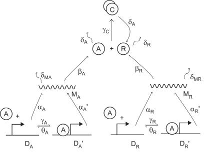
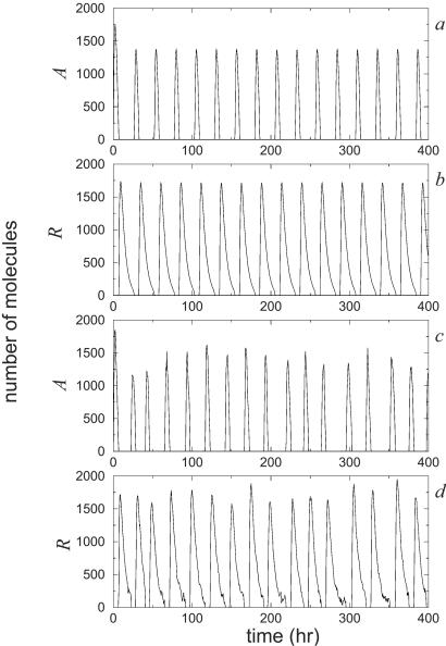
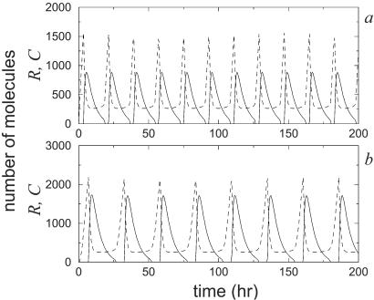
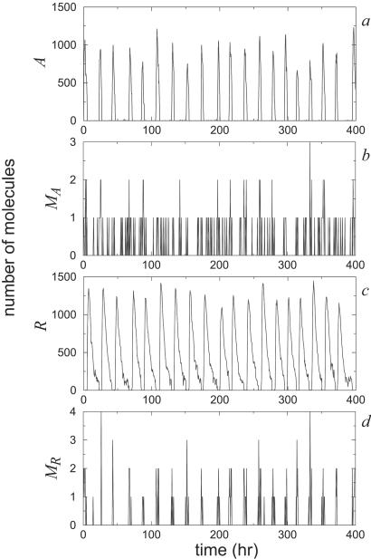
A wide range of organisms use circadian clocks to keep internal sense of daily time and regulate their behavior accordingly. Most of these clocks use intracellular genetic networks based on positive and negative regulatory elements. The integration of these "circuits" at the cellular level imposes strong constraints on their functioning and design. Here, we study a recently proposed model [Barkai, N. & Leibler, S. (2000) Nature (London), 403, 267-268] that incorporates just the essential elements found experimentally. We show that this type of oscillator is driven mainly by two elements: the concentration of a repressor protein and the dynamics of an activator protein forming an inactive complex with the repressor. Thus, the clock does not need to rely on mRNA dynamics to oscillate, which makes it especially resistant to fluctuations. Oscillations can be present even when the time average of the number of mRNA molecules goes below one. Under some conditions, this oscillator is not only resistant to but, paradoxically, also enhanced by the intrinsic biochemical noise.
Figures
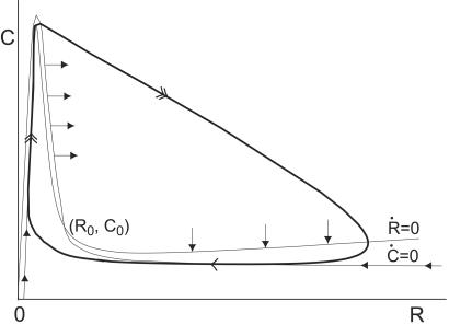
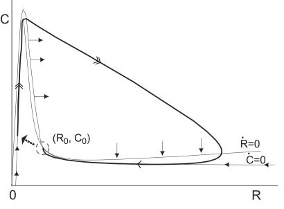
 dR/dt = 0 and Ċ
dC/dt = 0 are the R and
C nullclines, respectively. The solid arrows give the
orientation of the direction field on the nullclines.
dR/dt = 0 and Ċ
dC/dt = 0 are the R and
C nullclines, respectively. The solid arrows give the
orientation of the direction field on the nullclines.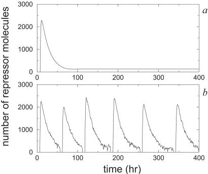
References
-
- Edmunds L N. Cellular and Molecular Bases of Biological Clocks. New York: Springer; 1988.
-
- Dunlap J C. Cell. 1999;96:271–290. - PubMed
-
- Barkai N, Leibler S. Nature (London) 2000;403:267–268. - PubMed
-
- McAdams H H, Arkin A. Trends Genet. 1999;15:65–69. - PubMed
-
- van Kampen N G. Stochastic Processes in Physics and Chemistry. Amsterdam: North−Holland; 1981.
Publication types
MeSH terms
Substances
LinkOut - more resources
Full Text Sources
Molecular Biology Databases
