Contrasting patterns of receptive field plasticity in the hippocampus and the entorhinal cortex: an adaptive filtering approach

Abstract

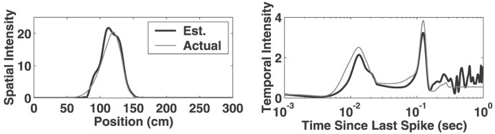
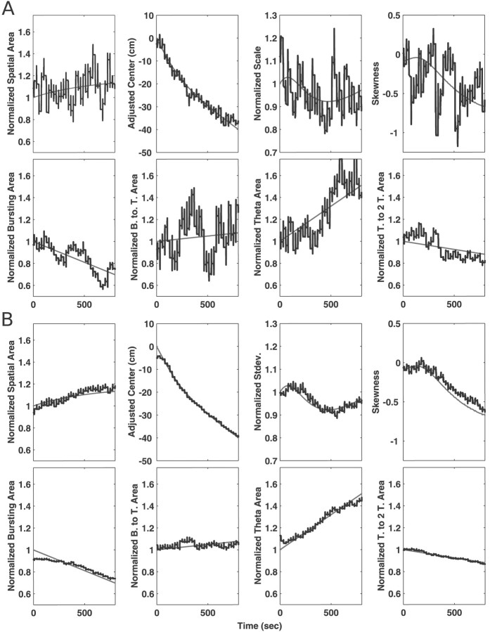
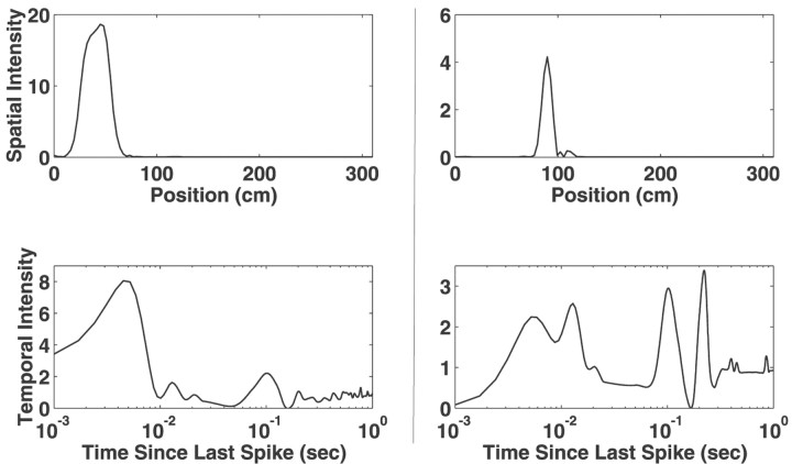
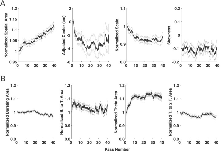
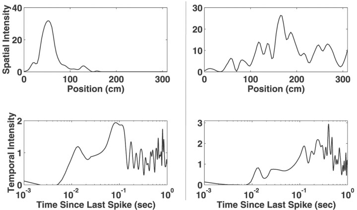
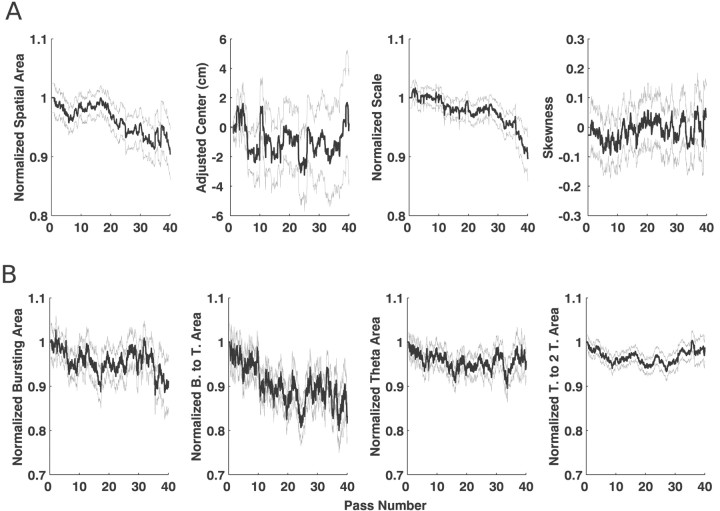
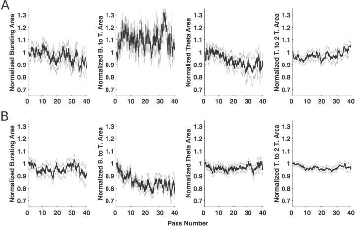
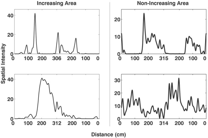
Neural receptive fields are frequently plastic: a neural response to a stimulus can change over time as a result of experience. We developed an adaptive point process filtering algorithm that allowed us to estimate the dynamics of both the spatial receptive field (spatial intensity function) and the interspike interval structure (temporal intensity function) of neural spike trains on a millisecond time scale without binning over time or space. We applied this algorithm to both simulated data and recordings of putative excitatory neurons from the CA1 region of the hippocampus and the deep layers of the entorhinal cortex (EC) of awake, behaving rats. Our simulation results demonstrate that the algorithm accurately tracks simultaneous changes in the spatial and temporal structure of the spike train. When we applied the algorithm to experimental data, we found consistent patterns of plasticity in the spatial and temporal intensity functions of both CA1 and deep EC neurons. These patterns tended to be opposite in sign, in that the spatial intensity functions of CA1 neurons showed a consistent increase over time, whereas those of deep EC neurons tended to decrease, and the temporal intensity functions of CA1 neurons showed a consistent increase only in the "theta" (75-150 msec) region, whereas those of deep EC neurons decreased in the region between 20 and 75 msec. In addition, the minority of deep EC neurons whose spatial intensity functions increased in area over time fired in a significantly more spatially specific manner than non-increasing deep EC neurons. We hypothesize that this subset of deep EC neurons may receive more direct input from CA1 and may be part of a neural circuit that transmits information about the animal's location to the neocortex.

Fig. 1.

Examples of changing spatial and temporal intensity functions used for simulation studies. Theleft shows the initial and final values for the spatial intensity functions from S2, and the right shows the initial and final values for the temporal intensity functions from T2. The dots superimposed on the curves represent control points.

Fig. 2.

A comparison of the estimated and actual spatial and temporal intensity functions. In the left(spatial intensity) and right (temporal intensity)plots, the gray lines represent the underlying spatial and temporal driving functions, respectively, used to generate a set of observed spike data as described above. In this example, the driving functions were a slowly skewing shifting Gaussian spatial intensity (a shifted version of S2) and fixed ISI modulation functions (T1). The spline estimates of these intensity functions, obtained by applying our adaptive estimation algorithm to this simulated spike train data, are displayed in the corresponding plot as black lines. Overall, the agreement between the actual and estimated functions is very good. The largest apparent deviations are in the temporal intensity function at long interspike intervals. This is attributable to the very small number of long ISIs and the corresponding lack of sampling of these intervals.

Fig. 3.

Examples of tracking from simulation S2–T2. In each plot, the gray line shows the actual trajectory of the measure, and the thicker black line shows the measure derived from the algorithm. Because our interest was in accurately capturing the trends in the data, we plotted the spatial area and scale measures, as well as all of the temporal measures, on a normalized scale. To construct these plots, we normalized the actual statistic by its mean and shifted it to start at one. We similarly normalized the estimated statistic by its mean and shifted it by the same amount as for the actual statistic. This produces plots in which changes are expressed as a proportion of the initial value. To construct the adjusted center plots, we also shifted the actual center curve to begin at zero and shifted the estimated curve by the same amount as the actual curve, so the two could be easily compared.A, Examples of the tracking of measures of the spatial and temporal intensity functions from a single simulated cell. Thetop row shows the spatial measures, and the bottom row shows the temporal measures. The tracking of the spatial area was somewhat noisy because of variability of the spike train and our choice of a learning rate that could track very fast changes, but nevertheless the trend captured by the estimate is similar to that present in the real data. The tracking of the center was very accurate. The tracking of the scale and the skewness were also, like that of the area measure, somewhat noisy, but once again the trends in the estimate follow the actual trends. Similarly, the trends in the measures of area under different sections of the temporal intensity curve were similar to the actual trends. B, The same measures averaged over 100 simulations. The trajectory of the normalized area, adjusted center, and normalized scale are all very close to the actual trajectories. The small deviation visible at the start of the area and center measures is attributable to the first pass estimate. The skewness also tracked well, although there were slightly larger errors for the skewness than for the area or the mean. The algorithm was also able to simultaneously track the trends in the different regions of the temporal function. The estimates of the burst-to-theta (21–75 msec) and theta to two-theta (150–300 msec) area were essentially identical to those for the actual function, and the estimates for the burst (1–21 msec) and theta (75–150 msec) regions follow the true values very closely, with a slight deviation at the beginning that was, as with the area and mean, related to the algorithm used to determine the first pass estimate. Thus, the algorithm is able to track changes in both the spatial receptive field and in the interspike interval structure of spike train data.

Fig. 4.

Examples of Komologorov–Smirnov plots showing the agreement between the statistical model and the data for CA1 and deep EC neurons. The plots were constructed as described in Materials and Methods. The top row shows the results when the model contained only an adaptive spatial component (e.g., the initial temporal intensity function was everywhere set to one and the temporal learning rate was set to zero), and the bottom rowshows the results when the model contains both adaptive spatial and temporal components with a temporal learning rate of 0.15. In both cases, the spatial learning rate was 2.0. Each plot shows the correct distribution (solid gray line), the 95% confidence intervals for the correct distribution (gray dashed lines), and the distribution resulting from the adaptive model (black line). Each column shows the results for a single cell in two conditions. Although the spatial function changes over time, the agreement between the model and the data is poor, suggesting that the model does not accurately capture the firing rate of the spike train. The plots for the CA1 neurons suggest that the lack of fit is most pronounced for low z_kvalues, which correspond primarily to shorter ISIs (Barbieri et al., 2001), suggesting that the model predicts fewer short intervals than are present in the data. In contrast, the plots for the deep EC neurons show lack of fit for the short intervals, which suggests that the model predicts more short intervals than were present in the data. The relative scarcity of short intervals is most likely to be attributable to the pronounced refractory period of most deep EC neurons (Frank et al., 2001). The bottom rowshows the plots when the model includes adaptive spatial and temporal components. When the model includes both components, the fit to the data is much improved, and, even when the model distribution lies outside of the 95% confidence intervals, it is nevertheless much closer to them than without the temporal intensity function.

Fig. 5.

Examples of instantaneous estimates of the spatial and temporal intensity functions from two CA1 neurons. Eachcolumn represents the functions for a single neuron. The spatial receptive fields of these two neurons are both sharply peaked, although their widths differ. The temporal intensity functions for the two neurons are very different, suggesting that the interspike interval structure of their spike trains differ. The neuron whose intensity function is shown on the left, for example, has a very large peak at ∼5 msec, indicating that this neuron has a strong tendency to fire in bursts. The intensity function on the right has two peaks at low intervals, suggesting that this neuron fires in three spike bursts. In addition, this intensity function has sharp peaks at ∼110 and 220 msec, indicating that the neuron fires frequently at the period of the theta rhythm and on alternating periods of the theta rhythm. These peaks correspond to interspike intervals that occurred frequently, and the peaks were present throughout the run, suggesting that they are consistent features of the temporal intensity function. These plots provide an easily interpretable summary of the firing properties of the neurons at each moment in time, and videos that show the evolution of these functions provide a powerful tool for examining the evolution of receptive fields.

Fig. 6.

Mean and SEs for the estimates of the spatial and temporal statistics for CA1 neurons. The black line in eachplot represents the trajectory of the mean for the statistics, and the gray lines represent the mean ± SE. The units on the x-axis are passes, in which one pass corresponds to the animal moving from one end of the U track to the other. The values on the y-axis are, for all statistics except the spatial mean and skewness, normalized to express the change in terms of the proportion of the initial value. The spatial means have been adjusted to start at 0 cm. A, The trajectories of the statistics for the spatial function. The area shows a clear and consistent increasing trend while the mean moves backwards over time. The scale also shows a clear decreasing trend, indicating that, even as the spatial intensity function increases in area, it decreases in extent, suggesting that, on average, CA1 activity becomes more spatially localized over time. Finally, the skewness measure had a consistently negative value but did not show a trend. These results are generally consistent with previous findings for CA1 cells.B, The trends for the temporal statistics. The burst (1–21 msec) region and the theta to two-theta regions (150–300 msec) showed little change, and the burst-to-theta region (21–75 msec) showed a small initial increase, followed by a return to baseline. In contrast, the theta region (75–150 msec) showed a rapid increase of ∼10%. That increase is consistent with the predictions of the model proposed by Mehta et al. (2000).

Fig. 7.

Examples of instantaneous estimates of the spatial and temporal intensity functions from two deep EC neurons. Eachcolumn represents the functions for a single neuron. The spatial intensity functions illustrate the variety of spatial receptive fields shapes found in the deep EC. The temporal intensity functions of deep EC neurons reflected the very small number of intervals <10 msec and generally had a peak near 120 msec, the period of the theta rhythm. Once again, the variability present in the portion of the temporal intensity function corresponding to larger ISIs (>300 msec) is attributable to the infrequent sampling of this region.

Fig. 8.

Mean and SEs for the estimates of the spatial and temporal statistics for CA1 neurons. The black line in eachplot represents the trajectory of the mean for the statistics, and the gray lines represent the mean ± SE. A, The trajectories for the statistics of the spatial function. Unlike CA1 neurons, the spatial intensity functions of deep EC neurons tended to decrease in area by ∼6% over the course of 40 passes. The mean of the spatial intensity function also showed no tendency to move backward, and no trends were found for the skewness. There was also a decrease of ∼7% in the scale, suggesting that the fields become somewhat more concentrated over time. B, The trajectories for the statistics of the temporal function. All regions of the temporal intensity function showed decreases, but the decrease was significant only for the burst-to-theta region in which the decrease averaged 9%. Thus, the decrease in the spatial area of the intensity function was associated with a relatively large decrease in the burst-to-theta region of the intensity function. When the model was run without a temporal intensity function, the spatial area decreased by ∼15%, indicating that the combination of spatial and temporal function declines results in the decrease of ∼15% in the firing rate of these neurons over 40 passes through the environment.

Fig. 9.

The temporal intensity functions for the increasing and non-increasing groups of deep EC neurons. Deep EC neurons were split into two groups based on the change observed in their spatial intensity function, one whose spatial area increased by at least 20% and another whose spatial area increased by <20% or decreased. A, The temporal intensity functions for the increasing group. B, The temporal intensity functions for the non-increasing group. Once again, the burst-to-theta (21–75 msec) region showed by far the greatest changes, with a small but nonsignificant increase in the case of the increasing group and a large, significant decrease of ∼14% for the decreasing group. Thus, the difference in spatial receptive field change between these two groups are associated primarily with changes in the propensity for these neurons to fire in intervals of 21 to 75 msec. Unfortunately, little is known about the physiology of neural circuitry in the deep EC, so these results are, at present, difficult to relate to a specific mechanism.

Fig. 10.

Examples of instantaneous receptive fields from deep EC neurons with increasing (left column) and non-increasing (right column) spatial intensity function areas. Each plot represents the spatial intensity function of a single deep EC neuron. On average, the neurons with increasing spatial intensity functions had more restricted spatial receptive fields than neurons with non-increasing spatial intensity functions.

References

1. Alonso A, Garcia-Austt E. Neuronal sources of theta rhythm in the entorhinal cortex of the rat. II. Phase relations between unit discharges and theta field potentials. Exp Brain Res. 1987;67:502–509. - PubMed
1. Amaral DG, Witter MP. Hippocampal formation. In: Paxinos C, editor. The rat nervous system. Academic; New York: 1995. pp. 443–493.
1. Barbieri R, Quirk MC, Frank LM, Wilson M, Brown EN. Construction and analysis of non-Poisson stimulus response models of neural spike train activity. J Neurosci Methods. 2001;105:25–37. - PubMed
1. Barnes CA, McNaughton BL, Mizumori SJ, Leonard BW, Lin LH. Comparison of spatial and temporal characteristics of neuronal activity in sequential stages of hippocampal processing. Prog Brain Res. 1990;83:287–300. - PubMed
1. Brown EN, Frank LM, Tang D, Quirk MC, Wilson MA. A statistical paradigm for neural spike train decoding applied to position prediction from ensemble firing patterns of rat hippocampal place cells. J Neurosci. 1998;18:7411–7425. - PMC - PubMed
Publication types
LinkOut - more resources