Three-dimensional image reconstructions of the contractile tail of T4 bacteriophage

Abstract

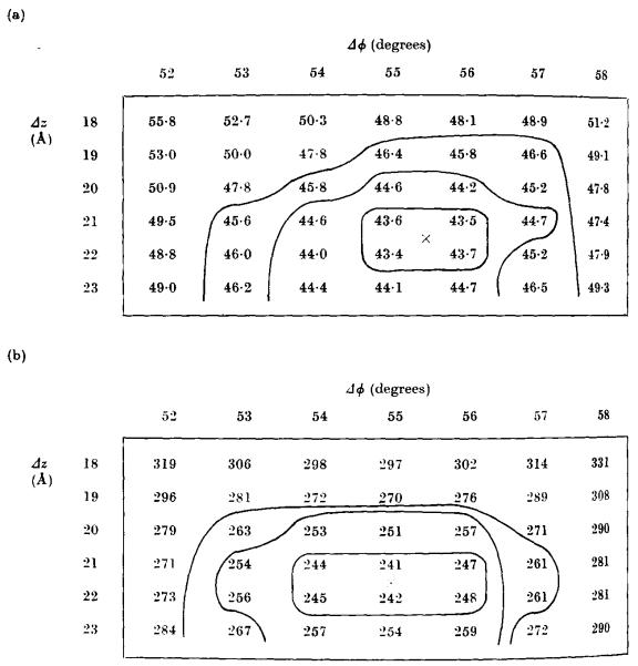
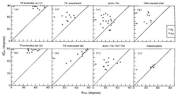
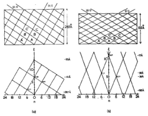
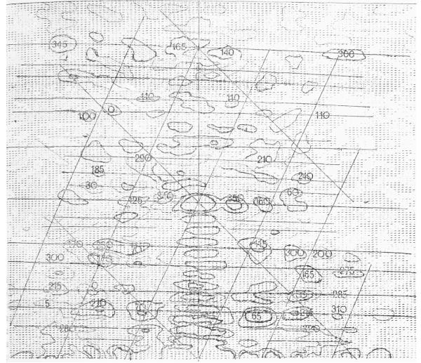
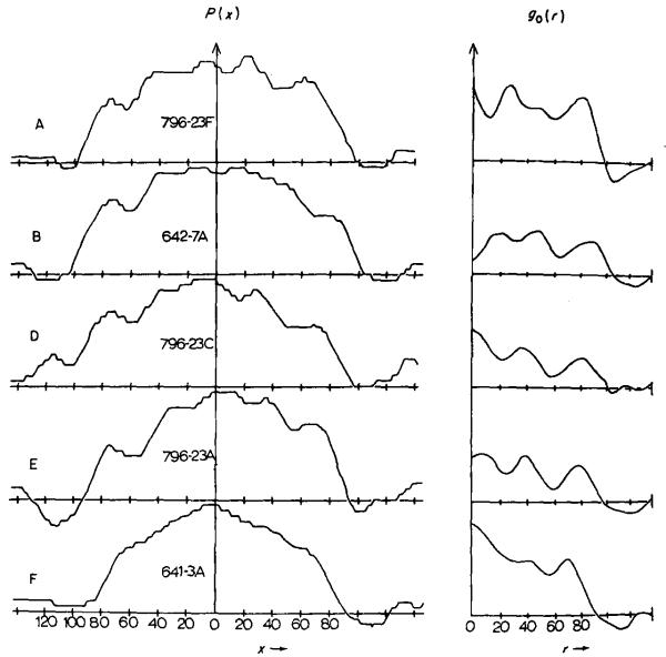
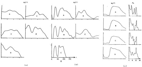
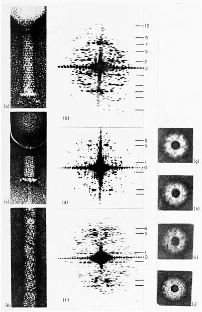
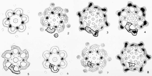
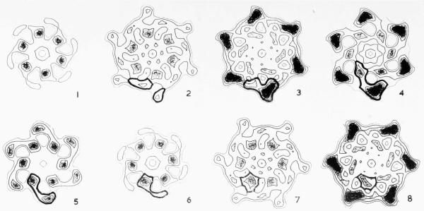
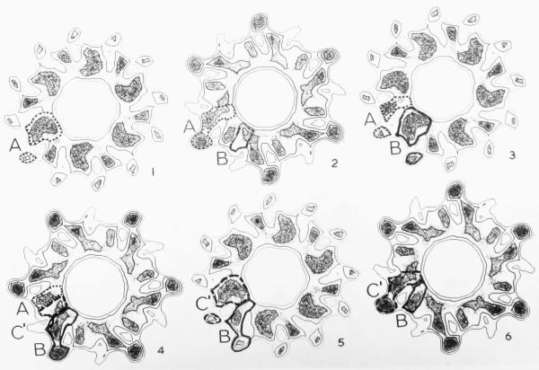
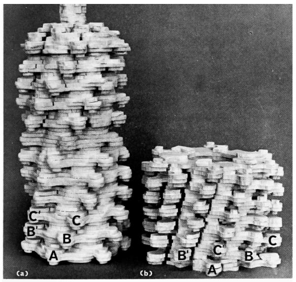
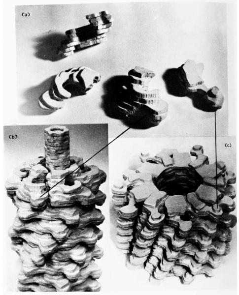
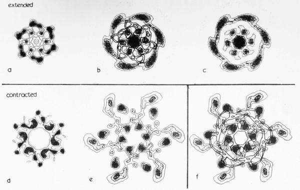
The three-dimensional structures of the extended T4 phage tail and polysheath, an aberrant form of the contracted tail sheath, have both been reconstructed from electron micrographs. The reconstructed map of the extended structure is at a somewhat higher resolution (~20 Å) than an earlier reconstruction, allowing tentative boundaries to be drawn between the individual protein subunits in the tail sheath. This improvement has been achieved by testing the degree of correlation between data from different images as part of the selection procedure and averaging the most highly correlated sets of data. Details of the correlation are given in the Appendix. The resolution of the map of the contracted structure is lower than that of the extended tail, in spite of a similar averaging of several images, because of the higher degree of distortion in this structure. Nevertheless, it has been possible, to some extent, to trace the changes in conformation of the subunit during contraction.

Fig. A1

Regions of typical residual maps close to the minimum values. In this case the residual maps were calculated by comparing the near-side data from an extended phage tail (particle F in Table A1) with the average from six nets of data, (a) The phase residual R(Δϕ,Δz), weighted as described in the text; (b) the least-squares residual S(Δϕ,Δz).

Fig. A2

Polarity plots for different sets of layer line data. The results (R_min) of correlating the phases of each set of data with those of a reference data set are plotted against the equivalent result ($R_{\text{min}}^{\ast }$) obtained with the reference turned upside down. The results for a non-polar structure should lie close to the diagonal line (e.g. (h) haemocyanin). For polar structures ((a) to (g)) the distance of the points above the diagonal line provides an indication of the degree of polarity present in the data, (a) Extended phage tail (1), was calculated by correlating each set of data with a chosen individual set. (b) Extended phage tail (2), was the result of correlating each data set with the average data. Notice the significant reductions in R_min, indicating a reduction in random error in the average, while the values of $R_{\text{min}}^{\ast }$ remain much the same as before. The results shown for the other structures ((c) to (g)) were obtained by correlating against their average data sets. The small arrows on the ordinate of each plot indicate the average values of the 2-fold residual (see text) which are closely similar to the corresponding values of $R_{\text{min}}^{\ast }$. For (a) and (b), see Table A1; for (c) and (d), see Table A2; for (e) and (f), see Wakabayashi et al. (1975); and for (g) and (h), see Table A3. TMV, tobacco mosaic virus; Tm, tropomyosin; TnT, troponin T; TnI, troponin I.

Fig. 1

(a) Surface lattice of the extended phage tail. The 6-start families of helices are labelled (0,1) and (1,1) according to the notation of Moody (1973). In the more conventional notation of Klug et al. (1958) for helical surface lattices, these are referred to as (6̅,5) and (6,2), respectively, Successive rings of subunits are labelled with different letters. The lattice is shown with a repeat after exactly seven rings, but moat specimens show small deviations from this: the (0,1) lattice lines (Moody’s “transitional helices”) tend to follow a slightly steeper angle, the (1,1) lines a slightly shallower angle. The annulus spaoing of 41 Å in the extended tail was determined by X-ray diffraction of tail cores (Moody, 1971b), which have been shown by optical diffraction of electron micrographs (Moody, 1971a) to have the same axial spacing as the extended tail sheath. The hand of the lattice has been determined by freeze-etching, by Bayer & Remsen (1970). (b)(n,l) plot showing the reciprocal lattice of the extended phage tail. For the lattice shown, the selection rule is l = −2n + 7m (where n must be a multiple of 6), although this is only an approximation to the real lattice. (c) Surface lattice of the contracted phage tail and polysheath which repeats after eleven rings of six subunits. The labelled subunits correspond to those with similar labels in the extended lattice (a), to show the change in relationship between neighbouring subunits during contraction. The “transitional” (0,1) helices of the extended tail have become the “short pitch” (0,1) helices (Moody, 1973). By coincidence, the helical notation is still (6̅,5) for the latter set of helices, although the (1,1) helices have become (6,6) in helical notation. The axial spacing of the annuli in polysheath was also determined by Moody (1967a), who calibrated the optical diffraction patterns from electron microscope images. The hand of the lattice was determined by Bayer & Remsen (1970). (d) (n,l) plot showing the reciprocal lattice of the contracted tail. The transformation which takes place in the helical surface lattice during contraction is accompanied by a similar lattice transformation (but rotated by 90°) in reciprocal space. The selection rule is l = n + 11m.

Fig. 2

A computer printout of the amplitudes of the computed Fourier transform of an extended T4 tail (particle F), which was densitometered on a raster with a spacing equivalent to about 5 Å. The amplitude peaks have been contoured at a relatively high level at low resolution but at a lower level at high resolution where the background is also much lower. The calculated phases of the main peaks are shown superimposed on them. Lines have been drawn through what appear to be the centres of the layer lines, and the “near side” helical surface lattice has been drawn in roughly to identify the peaks on the layer lines. The 1st, 6th, 8th and 13th layer lines are “split” into two because the longitudinal repeat distance is not exactly 7 annuli as drawn in Fig. 1. The selection rule in this case can be expressed approximately as l = −2n + 6·9m.

Fig. 3

A comparison of the radial density distributions calculated from different individual extended tails. The left-hand curves are the mean projected densities across each image, averaged along the axis. B and F are the most symmetrical and, of these two, B appears to be the best, since a dip presumably corresponding to the centre of the tail core is resolved at the centre of the density distribution. The right-hand curves are the mean radial density distributions of the three-dimensional reconstructed images, calculated by Fourier–Bessel transformation of the equatorial data in the Fourier transforms of the original images. The curves all have similar features (i.e. three peala at roughly the same radii) but B appears to be the best; it shows a minimum at the centre corresponding to the hole in the tail core.

Fig. 4

Calculations of the mean radial density distribution for contracted tail and polysheath. (a) Radial density distributions calculated from equatorial data of individual polysheath transforms. Although they are fairly similar near the outside, at inner radii they vary wildly. (b) Radial density distributions calculated from the equatorial data of individual contracted tails seen side-on, most of whioh still contained a central core. Four of the curves show a peak at 16 to 45 Å, which represents the wall of the core. The sheath is represented by a double peak in most cases. (c) Mean radial density distributions calculated from contracted sheaths seen end-on on the electron microscope grid, after being separated from their capsid, baseplate and tail core (see Plate I(g) to (j)). The rotational power spectra (Crowther & Amos, 1971) on the far right are a guide to whether or not the view is exactly down the axis. A direct view of an undistorted specimen should give peaks at n = 0, n = 6 and n = 12, but not in between. Since the images did not have very strong azimuthal modulations, the peak at n = 0 is much larger than the other peaks. The last example was considered to be reasonably good and was used in the three-dimensional image reconstructions of the contracted tail and polysheath, after being scaled to a similar level to the radial density distributions caloulated from side-on views ((a) and (b)).

Plate I

Electron microscope images of T4 bacteriophage tail structures, negatively stained with uranyl acctate, and optical diffraction patterns obtained from them. (a) An extended tail (Magnification 100,000×). (b) Optical diffraction pattern of (a). The layer lines are numbered according to the selection rule l = −2n + 7m, where n may only have values that are multiples of six (DeRosier & Klug, 1968). The seventh layer line arises from the 41 Å spacing of the stacked rings of subunits in the extended tail. Layer lines out to l = 14 (20 Å) can be identified in the computed Fourier transform although the signal to noise ratio is very low. In the optical transform shown here the 12th layer line (24 Å) is the last that can be detected (best seen in the lower half of the pattern). (c) A contracted tail showing the core pushed out through the baseplate. Magnification 100,000×. (d) Optical diffraction pattern of (c). The selection rule is now l = n + 11m (Moody, 1967a). The fifth layer line corresponds to a spacing of 38 Å. No layer lines beyond the sixth can be identified in either the optical or computed transforms. (e) A length of T4 polysheath. The strong transverse lines are stain-filled grooves between adjacent “short pitch” (0,1) helices (Fig. 1). Magnification 100.000×. (f) Optical diffraction pattern of (e), which indexes in the same way as the contracted tail pattern (Moody, 1967a). Layer lines beyond l = 6 could not be identified with certainty. (g) to (j) End-on views of contracted tails, used to determine the radial density distribution of contracted sheath, as shown in Fig. 4(c) ((g) = A, (h) = B, (i) = C, (j) = D).

Plate II

Sections normal to the helix axis through two average three-dimensional reconstructed images of the extended tail of T4. (Magnification 2,200,000×). (a) was calculated from averaged “near side” data, (b) from averaged “far side” data. The sections, which are viewed from the head end. are spaced at intervals of 8-2 Å along the axis, so that they repeat after five sections. They are numbered in increasing order from baseplate to capsid. High density represents protein. The contours have been drawn at regular intervals above a lower cut-off level and the peaks are shaded to distinguish them from holes. The resulting plots are thus combinations of the two ways of representing electron density described by Gossling (1967). The contours extend to a nominal radius of about 100 Å. The lowest contour level has been chosen to show clearly the hole in the centre of the tail core and the helical tunnels at 70 Å radius. The proposed boundaries of a single subunit of the sheath are shown as thicker lines superimposed on the contoured sections. They have been chosen to cut through the weaker parts of the map wherever possible. The axial range of the supposed subunit covers more than one 41 Å annulus, since it is slightly tilted. It starts at an outer radius in section 2 and ends at an inner radius in section 8. The annulus of subunits below ends in section 3, while the annulus above starts in section 7. Thus the boundary drawn in each section includes less than one-sixth of the total area. Three views of a three-dimensional model of the proposed subunit are shown in Plate V.

Plate II

Sections normal to the helix axis through two average three-dimensional reconstructed images of the extended tail of T4. (Magnification 2,200,000×). (a) was calculated from averaged “near side” data, (b) from averaged “far side” data. The sections, which are viewed from the head end. are spaced at intervals of 8-2 Å along the axis, so that they repeat after five sections. They are numbered in increasing order from baseplate to capsid. High density represents protein. The contours have been drawn at regular intervals above a lower cut-off level and the peaks are shaded to distinguish them from holes. The resulting plots are thus combinations of the two ways of representing electron density described by Gossling (1967). The contours extend to a nominal radius of about 100 Å. The lowest contour level has been chosen to show clearly the hole in the centre of the tail core and the helical tunnels at 70 Å radius. The proposed boundaries of a single subunit of the sheath are shown as thicker lines superimposed on the contoured sections. They have been chosen to cut through the weaker parts of the map wherever possible. The axial range of the supposed subunit covers more than one 41 Å annulus, since it is slightly tilted. It starts at an outer radius in section 2 and ends at an inner radius in section 8. The annulus of subunits below ends in section 3, while the annulus above starts in section 7. Thus the boundary drawn in each section includes less than one-sixth of the total area. Three views of a three-dimensional model of the proposed subunit are shown in Plate V.

Plate III

Sections normal to the helix axis through the average three-dimensional reconstructed image of T4 polysheath, including the radial density distribution from an end-on view of a contracted tail, which has produced the hole in the centre of the model. (Magnification 1,500,000×.) The sections are spaced at intervals of 8·7 Å along the axis, so that alternate sections are similar. They are viewed from what is thought to be equivalent to the capsid end of the structure and are numbered in increasing order from baseplate to capsid ends. The densities are represented by a combined contour and density plot, as in Plate II. The boundaries of the subunits are fairly obvious at the outermost radii, but are more difficult to distinguish at inner radii. The possible boundaries of three neighbouring subunits in different rings have been drawn in and labelled A (dotted boundary), B (thick solid lines) and C (dashed boundary). Continuity of the subunits from section to section has been used as a criterion in choosing the boundaries. Neighbouring annuli of subunits appear to interdigitate much more than in the extended structure, so that each section includes sections through at least 12 subunits. An isolated subunit constructed from these sections is shown in Plate V.

Plate IV

Views of models representing the three-dimensional reconstructed images of T4 extended tail and polysheath. Each model consists of 12 annuli and thus corresponds to half of a complete phage tail. The outer knobs of some of the subunits are labelled to show the lattice transformation (of Fig. 1). The upper surfaces of the models have been finished off in accordance with the interpretation of the subunit boundaries shown in Plates II and III, to represent the top surfaces of individual annuli of subunits. The subunits are shown in more detail in Plate V. In the model of the extended tail (a) a short continuation of the tail core is shown. Magnification 2,400,000×.

Plate V

(a) Models of individual subunits of extended and contracted sheath as interpreted in Plates II and III. Three views of the extended subunit and one of the contracted subunit (far right) are shown. Magnification 3,600,000×. (b) and (c) Close-up views of the models of the extended and contracted structures showing the three-dimensional relationships between the subunits in more detail. Magnification 3,000,000×.

Plate VI

Comparisons of sections of the extended phage tail and polysheath with baseplates in extended and contracted forms. Magnification 1,300,000×. (a) A section through the centre of an annulus of subunits in the near side three-dimensional reconstructed image (see Plate II(a)), viewed from above. This is fairly representative of the density distribution normal to the axis throughout the whole annulus. (b) Contours of the tail section shown in (a) superimposed on the filtered baseplate image shown in (c). The inner parts of the sheath subunits fit closely on to the central structure of the baseplate. (c) Rotationally filtered image of an extended baseplate (Crowther & Amos, 1971). The top surface of the baseplate is believed to have been in contact with the carbon substrate of the electron microscope grid, and therefore faces upwards in this print (R. A. Crowther, personal communication). (d) A section through the centre of an annulus of subunits in the polysheath three-dimensional reconstructed image (see Plate III), viewed from above. (e) Rotationally filtered image of a baseplate in the contracted form (J. King & R. A. Crowther, unpublished work). None of the polysheath sections in Plate III can be made to superimpose well on the baseplate image. (f) Contours of the extended baseplate superimposed on the contracted baseplate image. The central parts of the two structures are very similar although there are marked changes in density distribution at the periphery. The lack of transformation of the central structure during contraction explains the difficulty in fitting the sections of contracted sheath on to the baseplate image.

References

1. Amos LA, Klug A. J. Cell Sci. 1974;14:523–549. - PubMed
1. Arndt UW, Crowther RA, Mallett JFW. J. Scient. Instrum. 1968;1:510–516. - PubMed
1. Bayer ME, Remsen CC. Virology. 1970;40:703–718. - PubMed
1. Crowther RA. Phil. Trans. Roy. Soc. London. 1971;261:221–230. - PubMed
1. Crowther RA, Amos LA. J. Mol. Biol. 1971;60:123–130. - PubMed
LinkOut - more resources