Fine gating properties of channels responsible for persistent sodium current generation in entorhinal cortex neurons

Abstract

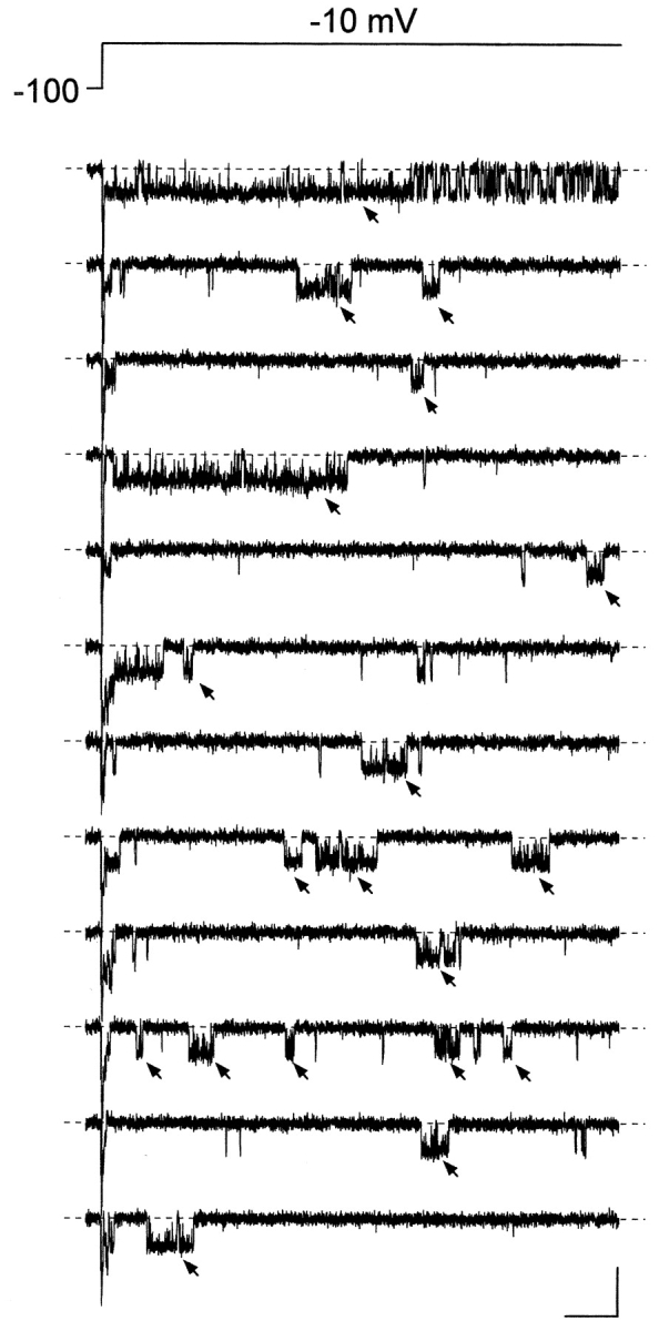
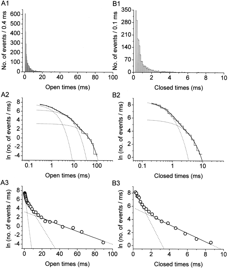
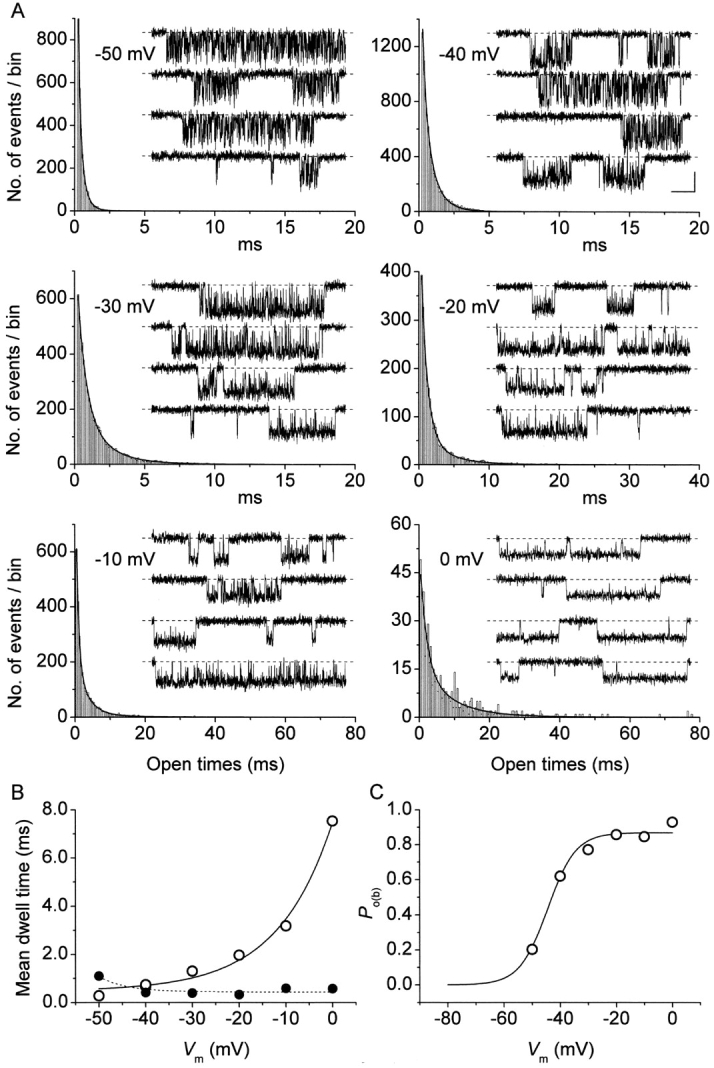
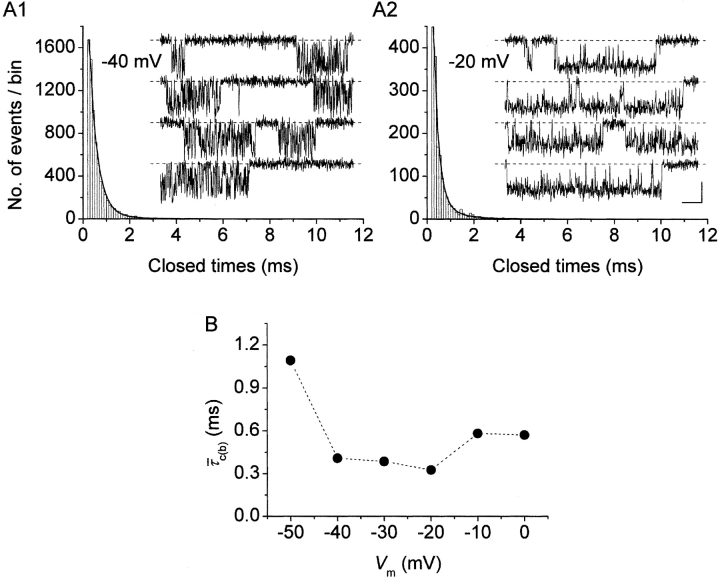
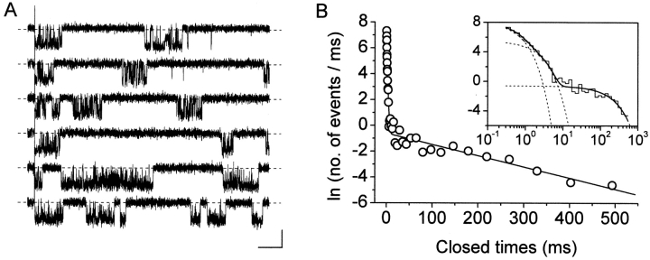
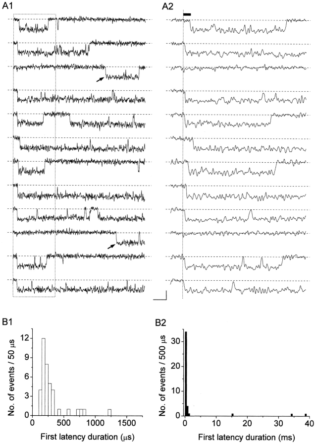
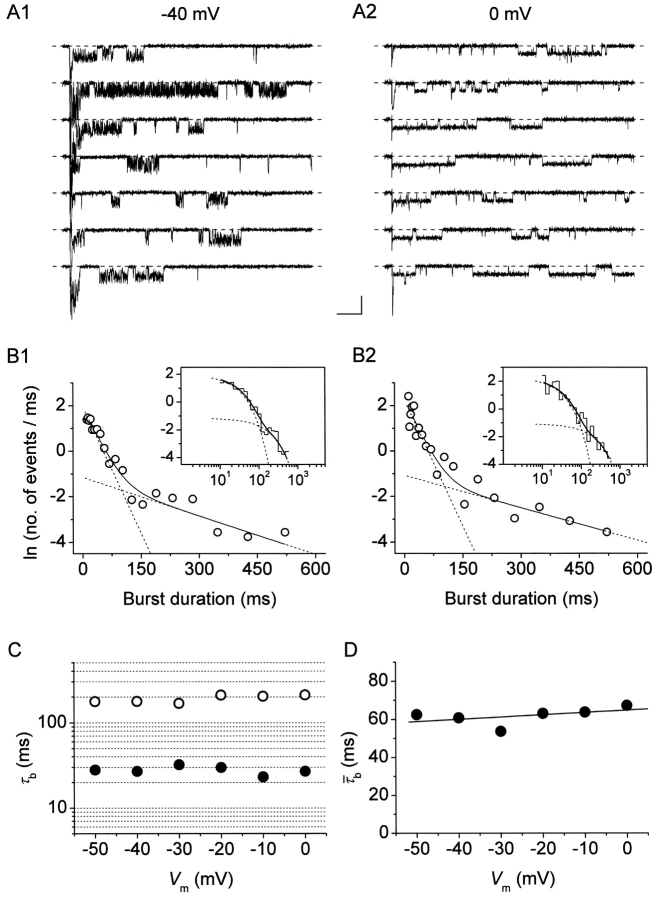
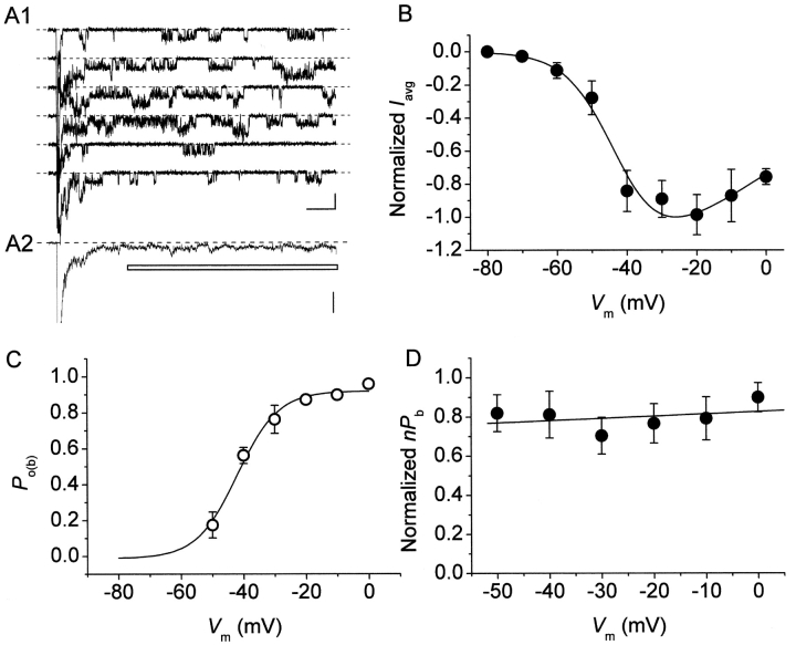
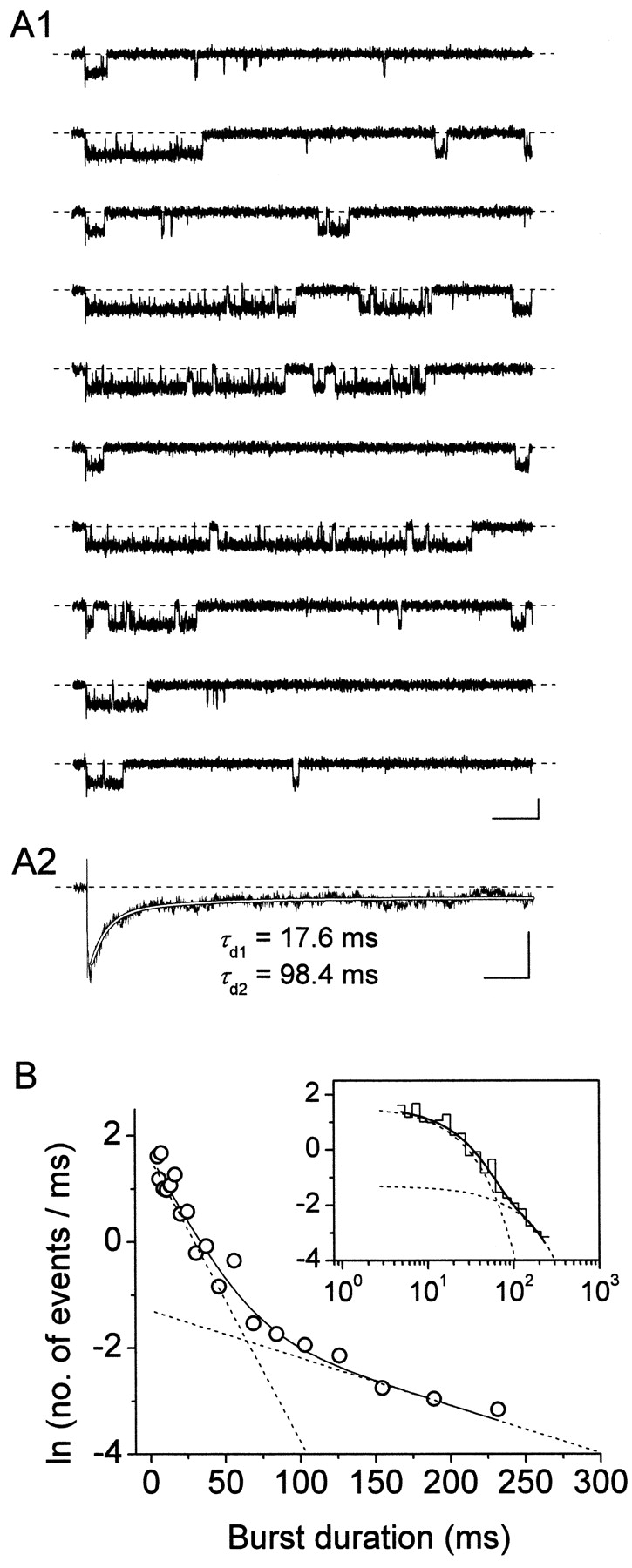
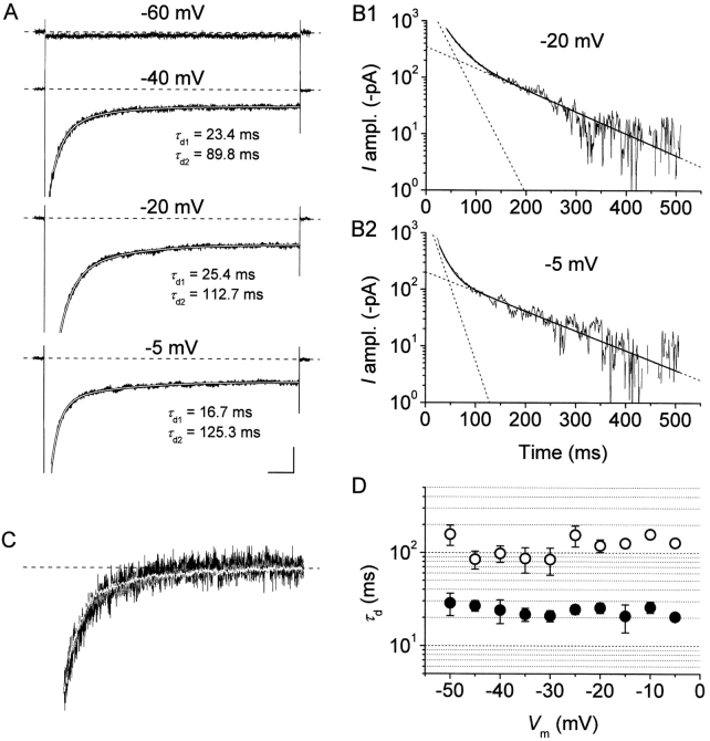
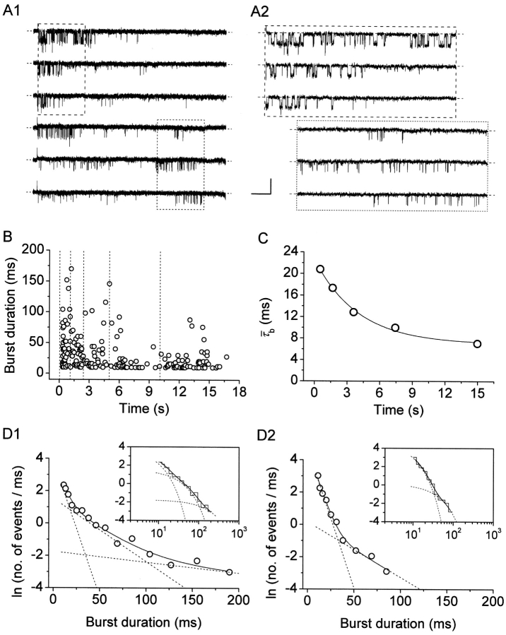
The gating properties of channels responsible for the generation of persistent Na(+) current (I(NaP)) in entorhinal cortex layer II principal neurons were investigated by performing cell-attached, patch-clamp experiments in acutely isolated cells. Voltage-gated Na(+)-channel activity was routinely elicited by applying 500-ms depolarizing test pulses positive to -60 mV from a holding potential of -100 mV. The channel activity underlying I(NaP) consisted of prolonged and frequently delayed bursts during which repetitive openings were separated by short closings. The mean duration of openings within bursts was strongly voltage dependent, and increased by e times per every approximately 12 mV of depolarization. On the other hand, intraburst closed times showed no major voltage dependence. The mean duration of burst events was also relatively voltage insensitive. The analysis of burst-duration frequency distribution returned two major, relatively voltage-independent time constants of approximately 28 and approximately 190 ms. The probability of burst openings to occur also appeared largely voltage independent. Because of the above "persistent" Na(+)-channel properties, the voltage dependence of the conductance underlying whole-cell I(NaP) turned out to be largely the consequence of the pronounced voltage dependence of intraburst open times. On the other hand, some kinetic properties of the macroscopic I(NaP), and in particular the fast and intermediate I(NaP)-decay components observed during step depolarizations, were found to largely reflect mean burst duration of the underlying channel openings. A further I(NaP) decay process, namely slow inactivation, was paralleled instead by a progressive increase of interburst closed times during the application of long-lasting (i.e., 20 s) depolarizing pulses. In addition, long-lasting depolarizations also promoted a channel gating modality characterized by shorter burst durations than normally seen using 500-ms test pulses, with a predominant burst-duration time constant of approximately 5-6 ms. The above data, therefore, provide a detailed picture of the single-channel bases of I(NaP) voltage-dependent and kinetic properties in entorhinal cortex layer II neurons.

Figure 1.

Persistent Na⁺ channel activity consists in prolonged and/or delayed burst openings. The figure shows twelve consecutive current sweeps recorded in response to 500-ms depolarizing pulses at −10 mV (top trace) in a representative cell-attached patch (patch A8716). The interpulse interval was 5.1 s. The arrows point to burst openings that were selected for analysis due to their characteristics (see the text for details). Calibration bars, 2 pA, 50 ms.

Figure 2.

Display and analysis of intraburst open- and closed-time data. (A) Frequency-distribution diagrams of intraburst open times at −10 mV. Data were collected from nine different patches. (B) Frequency-distribution diagrams of intraburst closed times at −10 mV. Data were from the same nine patches used for A. A1 and B1 show histograms constructed after linear binning of original data and displayed on a double-linear scale (bin width, 0.4 ms in A1; 0.1 ms in B1). A2 and B2 are log-log histograms. Data were binned logarithmically (11.4 bins/decade), and the natural logarithm of the numbers of observations per ms [ln(n/ms)] was plotted as a function of time in a logarithmic scale. Smooth, enhanced lines are third (A2) or second (B2) order exponential functions obtained by applying the fitting function of Eq. 1 (materials and methods). Smooth, dotted lines are the single exponential components shown separately. Fitting parameters are specified in Table I. A3 and B3 are log-linear plots of the same data. Data were binned logarithmically as above, and the quantity ln(n/ms) was plotted as a function of time in a linear scale. The x value of each point is the logarithmic midpoint of the corresponding bin. Continuous and dotted lines are the same functions as in the two previous panels: single exponential components appear here as straight lines.

Figure 3.

Open times are strongly voltage dependent. (A) Frequency distributions of open times at six different membrane potentials (−50 to 0 mV). Each histogram has been constructed pooling together data from 4 to 10 different patches. Data are shown binned linearly and plotted on a double-linear scale (bin width = 0.1 ms at −50 to −30 mV; 0.2 ms at −20 mV; 0.4 ms at −10 and 0 mV). Note the different time scales used. Smooth lines are best third order exponential fittings obtained applying Eq. 1 to log-log plots of the same data binned logarithmically (see materials and methods, and Fig. 2). Fitting parameters are specified in Table I. For each test potential, exemplary 210-ms current-trace segments were selected from 500-ms sweeps recorded in a single representative patch (patch B8708), and are shown in the inset of the corresponding panel (calibration bars: 1 pA, 25 ms). (B) Plot of mean open time (, calculated from fitting parameters as explained in the text) as a function of membrane potential (open circles). The continuous line is the best fitting to data points obtained applying the exponential function = A · exp(V _m/h) + C, which returned the following fitting parameters: A = 7.0 ms, h = 11.8 mV, C = 0.47 ms. Filled circles are mean intraburst closed times (: see Fig. 4) measured in the same patches, shown here for comparison. (C) Voltage dependence of average intraburst opening probability (P _o(b)), calculated from and as explained in the text. The continuous line is the best Boltzmann fitting to data points. Fitting parameters are: A = 0.869, V _1/2 = −44.5 mV, k = −5.02 mV.

Figure 4.

Intraburst closed times are scarcely voltage dependent. (A) Frequency distributions of intraburst closed times at two exemplary membrane potentials (−40 mV in A1, −20 mV in A2). The histograms have been constructed pooling together data from seven (−40) or nine (−20) different patches. Data are shown binned linearly and plotted on a double-linear scale (bin width = 0.1 ms). Smooth lines are the best second-order exponential fittings obtained applying Eq. 1 to log-log plots of the same data binned logarithmically (see the materials and methods, and Fig. 2). Fitting parameters are specified in Table I. For both test potentials, exemplary 100-ms current-trace segments were selected from 500-ms sweeps recorded in a single representative patch (patch D8716), and are shown in the inset of the corresponding panel over an expanded time scale (calibration bars: 1 pA, 10 ms). (B) Plot of mean intraburst closed time (, calculated from fitting parameters as explained in the text) as a function of membrane potential.

Figure 5.

Analysis of interburst closed times. (A) Selected 500-ms sweeps from a patch in which the activity of a single NaP channel was recorded in isolation (patch F8711). The traces have been chosen to show the occurrence of reopenings and illustrate inter-burst intervals. Test potential was −10 mV. Calibration bars, 1 pA, 50 ms. (B) Frequency distribution of total closed times at −10 mV. The graphs have been constructed pooling together data from two single-channel patches. Data were binned logarithmically and in the main panel are shown in a log-linear plot. In the inset, the same data are shown as a log-log histogram. In both panels, the smooth, continuous line is the best third-order exponential fitting obtained applying Eq. 1 to the log-log plot. Dotted lines are the single exponential components of the fitting function shown separately. Fitting parameters are: W ₁ = 1094.29, τ _c1 = 351.2 μs; W ₂ = 291.57, τ _c2 = 1.215 ms; W ₃ = 63.42, τ _c3 = 115.53 ms.

Figure 6.

Analysis of first latencies at −10 mV. (A) Selected sweeps showing persistent Na⁺ channel openings in isolation from a representative patch (patch H8710). Single-channel currents recorded in response to 50-ms depolarizing step pulses at −10 mV are shown in A1. A2 shows a detail, over an expanded time scale, of the first 15 ms of the same traces as in A1 (corresponding to the segments included in the dotted-line box of A1). The arrows in A1 remark two channel openings characterized by remarkably long first latencies. The filled bar in A2 indicates the first latency of the channel opening occurring in the top trace, determined starting from the depolarization's zero time point (dotted vertical line). Calibration bars, 1 pA, 5 (A1) or 1.5 (A2) ms. (B) Frequency distribution of first latencies at −10 mV. Data have been obtained in a total of 42 sweeps from two different patches, and are shown binned linearly and plotted on a double-linear scale. B1 highlights the initial part of the distribution (up to 1.75 ms). B2 shows the whole frequency distribution (with a different bin width).

Figure 7.

Analysis of burst duration. (A) Selected current traces recorded in response to 500-ms depolarizing pulses at −40 mV (A1) or 0 mV (A2) in a representative patch (patch D8708). Calibration bars, 2 pA, 50 ms. (B) Frequency distributions of burst duration at V _m = −40 mV (B1) and 0 mV (B2). Each graph has been constructed pooling together data from five different patches. Data were binned logarithmically and in the main panels are shown as log-linear plots. In the insets, the same data are shown as log-log histograms. In all panels, the smooth, continuous line is the best second-order exponential fitting obtained applying Eq. 1 to log-log plots. Dotted lines are the single exponential components of fitting functions shown separately. Fitting parameters are: W ₁ = 192.16, τ _b1 = 26.98 ms; W ₂ = 55.83, τ _b2 = 177.47 ms (−40 mV); W ₁ = 258.22, τ _b1 = 27.03 ms; W ₂ = 72.26, τ _b2 = 210.83 ms (0 mV). (C) Plot of burst-duration time constants (τ _bs) as a function of membrane potential. Filled and empty circles are τ _b1 and τ _b2 values, respectively. Note the logarithmic scale of the y axis. (D) Voltage dependence of mean burst duration (, calculated from fitting parameters as explained in the text).

Figure 8.

The probability of NaP channels to dwell in a “bursting state” is largely voltage-independent. (A) Measurement of I _NaP amplitude from ensemble-average currents (EACs). A1 shows exemplary traces recorded in response to 500-ms depolarizing pulses at −30 mV in a representative multichannel patch (patch C8703), A2 shows the trace obtained by averaging 20 such traces from the same patch. The horizontal bar marks the part of the trace the points of which were averaged to derive the amplitude of EAC's persistent component (I _avg). Calibration bars, 2 pA, 50 ms (A1); 1 pA (A2). (B) Plot of average I _avg amplitude, measured in EACs, as a function of membrane potential (n = 6). The continuous line is the best fitting to data point obtained applying the following function: I _avg = A/{1 + exp[(V _m – V _1/2)/k]} · (V _m – V _Na), were V _Na is the average, extrapolated reversal potential of persistent Na⁺-channel openings as derived from the same six patches (54.5 mV). Fitting parameters are: V _1/2 = −42.2 mV, k = −6.8 mV. (C) Values of intraburst opening probability (P _o(b)) were derived from each of the same six patches as in B, averaged, and plotted as a function of membrane potential. The continuous line is the best Boltzmann fitting to data points. Fitting parameters are: A = 0.92, V _1/2 = −42.0 mV, k = −6.6 mV. (D) Voltage dependence of average, normalized nP _b (see text). nP _b values were derived for the same six patches as in B and C.

Figure 9.

Burst-duration time constants result in very similar macroscopic relaxation time constants in ensemble-average traces. (A) Kinetic properties of the ensemble-average current derived, for the test potential of −10 mV, from patches showing the activity of single NaP channels in isolation. A1 shows exemplary traces recorded in response to 500-ms depolarizing pulses at −10 mV in the same patch as in Fig. 5, A2 shows the trace obtained by averaging 34 such traces from the two single-channel patches available. The smooth, blank line in A2 is the best biexponential fitting to data points (time-constant values are specified nearby). Calibration bars, 1 pA, 50 ms (A1); 400 fA, 50 ms (A2). (B) Frequency distribution of burst durations at −10 mV for the two single-channel patches illustrated above. The graphs have been constructed pooling together data from the same two patches used for A2. Data were binned logarithmically and in the main panel are shown in a log-linear plot. In the inset, the same data are shown as a log-log histogram. In both panels, the smooth, continuous line is the best second-order exponential fitting obtained applying Eq. 1 to the log-log plot. Dotted lines are the single exponential components of the fitting function shown separately. Fitting parameters are: W ₁ = 90.21, τ _b1 = 18.71 ms; W ₂ = 30.68, τ _b2 = 111.92 ms.

Figure 10.

I _NaP fast and intermediate decay time constants closely parallel burst-duration time constants characteristic of persistent Na⁺-channel openings. (A) Whole-cell Na⁺ currents recorded in response to 500-ms depolarizing pulses at four different test potentials in a representative neuron (cell 96315). The traces are shown to highlight the I _NaP component (part of the peak transient component at −40 to −5 mV has been blanked). The decay phases of the three lower traces (starting at 20–30 ms from the onset of the depolarizing test pulse) have been best fitted with a second order exponential function (smooth, blank lines). The time constants values returned by fittings are specified close to each trace. Calibration bars, 100 (−60 mV) or 200 (the remaining potentials) pA, 50 ms. (B) The two lower traces of A and the corresponding fitting functions are shown sign-inverted, subtracted of their offset components, and plotted on a logarithmic y axis to highlight the correspondence between second order exponential fitting functions and the experimental traces. Smooth, enhanced lines are the total fitting functions, dotted lines are the single exponential components shown separately. (C) Average I _NaP traces obtained from five cells for three different test potentials (−45 mV, black trace; −25 mV, blank trace; −5 mV, gray trace) are shown normalized in amplitude and superimposed to highlight the similarities in their decay kinetics. Current traces were subtracted of their offset components and normalized for the amplitude measured at 40 ms from the onset of the depolarizing test pulse (the parts preceding the above time point have been omitted). Same time scale as in A. (D) Voltage dependence of I _NaP “fast” and “intermediate” decay time constants (τ _d1 and τ _d2: filled and open circles, respectively) as obtained from the protocol illustrated in A and B (n = 5). Note the logarithmic scale of the y axis.

Figure 11.

Prolonged depolarizations induce longer interburst closings and shorter burst openings. (A) Single-channel recordings obtained applying long-lasting (20-s) depolarizing pulses at −20 mV in a representative patch (same patch as in Fig. 7 A). A1 shows six selected 20-s current sweeps in their entire length. 5-s segments were extracted from either the initial (dashed-line box) or the final (dotted-line box) part of the same sweeps, and shown in A2 over an expanded time scale to highlight the different mean duration of burst openings. Calibration bars, 2 pA, 2 s (A1) or 490 ms (A2). (B) Scatter plot of burst duration versus time during the application of 20-s depolarizing pulses at −20 mV. Data are from the same patch illustrated in A. Burst durations were plotted as a function of the starting point of each burst. The vertical, dotted lines mark the limits between the regions in which the plot was subdivided, and from each of which data values were extracted and used to construct burst-duration histograms (see D1 and D2). (C) Time course of mean burst duration, , during long-lasting (20-s) depolarizing pulses at −20 mV. Data points are values derived from burst-duration histograms (see D1 and D2) constructed for the five regions in which the experimental traces were subdivided (see B). The continuous line is the best exponential fitting to data points. Fitting parameters are: A = 15.61 ms, τ = 4.01 s, C = 6.95 ms. (D) Frequency distributions of burst duration in early (D1) and late (D2) phases of 20-s depolarizing pulses at −20 mV. Each graph has been constructed pooling together data from five different patches. The data shown in D1 and D2 were collected from the first and the last, respectively, of the periods in which burst-duration time courses were subdivided (see B). Data were binned logarithmically and in the main panels are shown as log-linear plots. In the insets, the same data are shown as log-log histograms. In all panels, the smooth, continuous line is the best third- (D1) or second- (D2) order exponential fitting obtained applying Eq. 1 to log-log plots. Dotted lines are the single exponential components of fitting functions shown separately. Fitting parameters are: W ₀ = 274.08, τ _b0 = 6.01 ms; W ₁ = 118.19, τ _b1 = 25.79 ms; W ₂ = 26.57, τ _b2 = 151.4 ms (D1); W ₀ = 612.28, τ _b0 = 5.83 ms; W ₁ = 34.09, τ _b1 = 29.26 ms (D2).

References

1. Agrawal, N., B.M. Hamam, J. Magistretti, A. Alonso, and D.S. Ragsdale. 2001. Persistent sodium channel activity mediates subthreshold membrane potential oscillations and low-threshold spikes in entorhinal cortex layer V neurons. Neuroscience. 102:53–64. - PubMed
1. Aldrich, R.W., D.P. Corey, and C.F. Stevens. 1983. A reinterpretation of mammalian sodium channel gating based on single channel recording. Nature. 306:436–441. - PubMed
1. Alonso, A., M. de Curtis, and R. Llinás. 1990. Postsynaptic Hebbian and non-Hebbian long-term potentiation of synaptic efficacy in the cortex in slices and in the isolated adult guinea pig brain. Proc. Natl. Acad. Sci. USA. 87:9280–9284. - PMC - PubMed
1. Alonso, A., and E. García-Austt. 1987. a. Neuronal sources of theta rhythm in the entorhinal cortex of the rat. I. Laminar distribution of theta field potentials. Exp. Brain Res. 67:493–501. - PubMed
1. Alonso, A., and E. García-Austt. 1987. b. Neuronal sources of theta rhythm in the entorhinal cortex of the rat. II. Phase relations between unit discharges and theta field potentials. Exp. Brain Res. 67:502–509. - PubMed