. 2002 Dec 15;22(24):10811-8.
doi: 10.1523/JNEUROSCI.22-24-10811.2002.

Isolation of relevant visual features from random stimuli for cortical complex cells

Affiliations

Isolation of relevant visual features from random stimuli for cortical complex cells

Jon Touryan et al. J Neurosci. .

Abstract

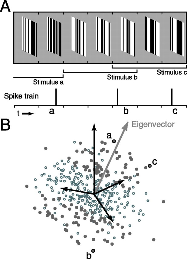
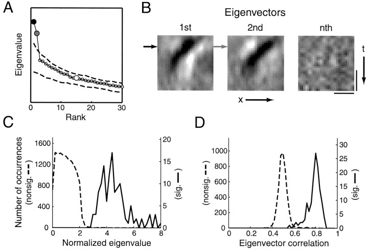
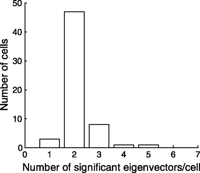
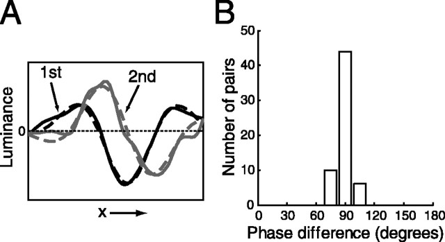
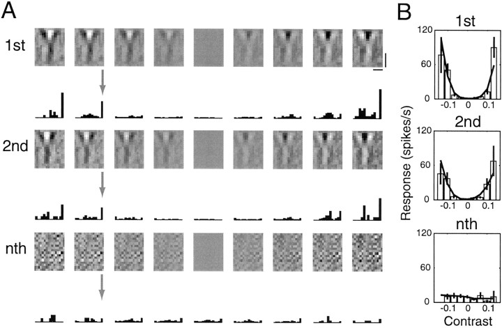
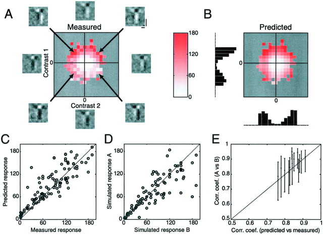
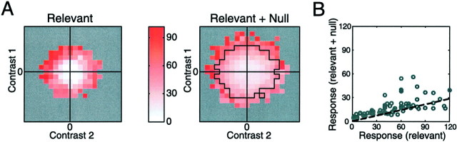
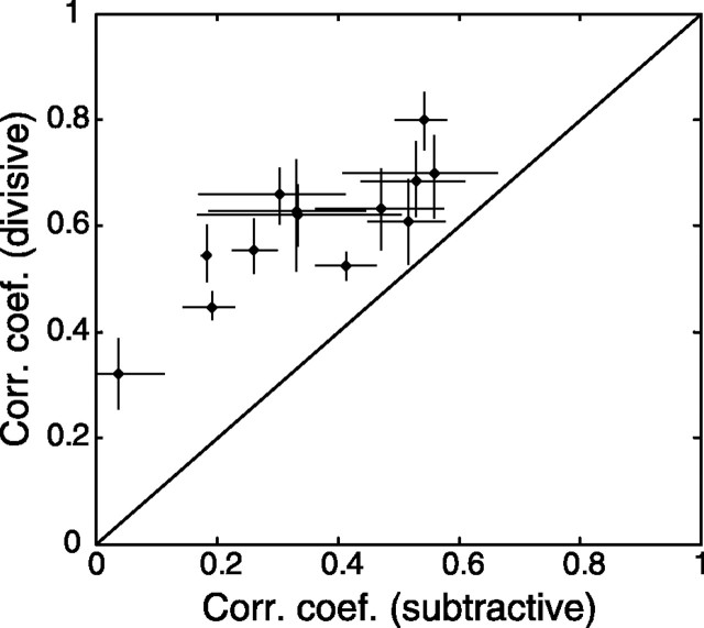
A crucial step in understanding the function of a neural circuit in visual processing is to know what stimulus features are represented in the spiking activity of the neurons. For neurons with complex, nonlinear response properties, characterization of feature representation requires measurement of their responses to a large ensemble of visual stimuli and an analysis technique that allows identification of relevant features in the stimuli. In the present study, we recorded the responses of complex cells in the primary visual cortex of the cat to spatiotemporal random-bar stimuli and applied spike-triggered correlation analysis of the stimulus ensemble. For each complex cell, we were able to isolate a small number of relevant features from a large number of null features in the random-bar stimuli. Using these features as visual stimuli, we found that each relevant feature excited the neuron effectively in isolation and contributed to the response additively when combined with other features. In contrast, the null features evoked little or no response in isolation and divisively suppressed the responses to relevant features. Thus, for each cortical complex cell, visual inputs can be decomposed into two distinct types of features (relevant and null), and additive and divisive interactions between these features may constitute the basic operations in visual cortical processing.


Figures

Fig. 1.
Fig. 1.
Illustration of a spike-triggered correlation analysis. A, Spatiotemporal random-bar stimuli (top) and the spike train response (bottom). Each bracket indicates a spatiotemporal stimulus pattern preceding a spike (for actual analysis, each pattern contained 16 rather than 3 frames). B, Schematic representation of the spike-triggered stimulus ensemble (filled circles) and the entire stimulus ensemble (open and filled circles) in a multidimensional parameter space. Each axis (black arrows) represents luminance at a particular bar position and time frame, and each point represents a stimulus pattern. Note that the actual stimulus ensemble is represented in a 256-dimensional space (16 frames by 16 bars). a–c indicate stimulus patterns shown in A. The gray arrow indicates an eigenvector of the spike-triggered ensemble with its eigenvalue (variance) greater than the eigenvalues of the entire ensemble.
Fig. 2.
Fig. 2.
Distinction between the significant and nonsignificant eigenvectors. A, The 30 largest eigenvalues of the spike-triggered correlation matrix of a complex cell. Dashed line, Control confidence interval (p = 10−4) obtained by random sampling of the entire stimulus ensemble (100 repeats; see Materials and Methods). Filled circles, Eigenvalues that are significantly different from the control; open circles, nonsignificant eigenvalues. B, Two significant eigenvectors (first and second) and one nonsignificant eigenvector (nth; n = 15 in this case) whose eigenvalues are indicated by the large circles in A. Arrow, 40 msec (the delay at which the spatial profiles of the eigenvectors are shown in Fig. 4A). Calibration: 1°, 100 msec.C, Distributions of significant (sig.;solid line) and nonsignificant (nonsig.;dashed line) eigenvalues from 60 complex cells. Each eigenvalue was normalized by the mean eigenvalue of the cell.D, Distribution of temporal correlation in significant and nonsignificant eigenvectors. The autocorrelation function of each eigenvector was computed along the temporal axis; the eigenvector correlation shown here was measured by the autocorrelation at the delay of 1 frame (16.7 msec) normalized by the autocorrelation at 0 delay, as follows:  x=116 t=116 V(x,t1)V(x,t)/x=116 t=116 V(x,t)V(x,t)+1/2,where V(x,t) represents the luminance value of the eigenvector at pixel x and temporal delayt (see Materials and Methods). This value provides a measure of the nonrandomness of the eigenvector structure between 0 (completely random) and 1 (temporally uniform).
Fig. 3.
Fig. 3.
Distribution of the number of significant eigenvectors found for each cell, from a total of 60 complex cells.
Fig. 4.
Fig. 4.
Relationship between the two most significant eigenvectors. A, Spatial profiles (solid lines) of the two significant eigenvectors shown in Figure2B at 40 msec from spiking (arrows) and their Gabor fits (dashed lines). The two Gabor fits had a phase difference of 90.4°. Dotted line represents mean luminance. B, Distribution of the spatial phase difference between the two significant eigenvectors of each complex cell.
Fig. 5.
Fig. 5.
Responses of a complex cell (different from that shown in Fig. 2) to individual features. A, Responses to two significant eigenvectors (first and second) and one nonsignificant eigenvector (nth, randomly chosen for each cell;n = 8 in this case). The top panel of each row shows the eigenvector presented at a range of positive (right) and negative (left) contrasts. Calibration: 1°, 100 msec. The PSTH in response to each stimulus is plotted below, with the arrow indicating the last time bin of the PSTH. B, Contrast–response function (amplitude of the last bin in each PSTH) for each vector (bars) and the fit of each side with a power function (line). Error bars indicate SEM.
Fig. 6.
Fig. 6.
Interaction between relevant visual features. A, Joint contrast–response function of a complex cell (different from Figs. 2 and 5), in which the amplitude of the response (color-coded, with the scale shown on theright in units of spikes per second) is plotted against the contrasts of both relevant features. The outer plotsdepict the stimulus patterns corresponding to selected points (indicated by arrows) in the contrast–response function. Calibration: 1°, 100 msec. The range of contrast represented in the center box is −0.33 to 0.33; the contrast of each feature varied at a step size of 0.033. Responses were measured only at contrasts at which the luminance signals in the movie do not exceed the range of the monitor. Gray indicates contrast at which the response was not measured. B, Prediction of the contrast–response function based on additive interaction between the two vectors. The left andbottom histograms represent the contrast–response functions for the first and second eigenvectors, respectively, computed from the joint contrast–response function in A in the following manner: For eigenvector 1, the response at each contrast (contrast 1) was computed by averaging the measured responses across all values of contrast 2 (average across each row). Similarly, the contrast–response function for vector 2 (bottom histogram) was computed by averaging the responses inA across all values of contrast 1. Prediction of the response at each combination of contrast 1 and contrast 2 was then made by summing the value in each of the histograms at the corresponding contrast. Predictions were made only for contrasts at which the actual responses were measured in A. C, Measured response in A plotted against the additive prediction inB at corresponding contrasts. Each circlerepresents data at one pair of contrasts. D, Response from one simulation (A) plotted against that from another (B) (see Materials and Methods).E, Correlation coefficients between simulated responses plotted against the correlation coefficient between the predicted and measured contrast–response functions for 13 complex cells.Vertical bars, 95% confidence intervals of correlation coefficients between simulated responses, with the mean indicated by the point (the mean is not in the middle of the bar, because the distribution of the correlation coefficient is skewed).
Fig. 7.
Fig. 7.
Suppressive effects of null features.A, Contrast–response functions of a complex cell for the two relevant features measured in the absence (left) or presence (right) of null features, with a luminance scale indicated in the middle (in spikes per second). The range of contrast represented in the boxes is −0.33 to 0.33. Contrasts of both features varied at a step size of 0.033. Theblack line in the right plot delineates the range of contrasts shown in the left plot. Higher contrasts for the relevant features were possible in the presence of null features, because the superposition of certain null features can reduce the extreme luminance values in the short movie to levels within the monitor limit. B, Responses in theleft plot versus the responses in the right plot in A at corresponding contrasts (in spikes per second). Each circle represents data at one pair of contrasts. The slope of the linear regression (dashed line) is 0.24.
Fig. 8.
Fig. 8.
Comparison between the subtractive and divisive models for null features. Correlation coefficients between the measured responses and the prediction based on the divisive model were plotted against the correlation coefficients between the measured responses and the prediction based on the subtractive model. Eachpoint represents the result of one cell. Error bar, 95% confidence interval, estimated using nonparametric bootstrap (see Materials and Methods for the Monte Carlo method used in the analysis).

Similar articles

Cited by

References

    1. Adelson EH, Bergen JR. Spatiotemporal energy models for the perception of motion. J Opt Soc Am A. 1985;2:284–299. - PubMed
    1. Albrecht DG, Geisler WS. Motion selectivity and the contrast-response function of simple cells in the visual cortex. Vis Neurosci. 1991;7:531–546. - PubMed
    1. Allman J, Miezin F, McGuinness E. Stimulus specific responses from beyond the classical receptive field: neurophysiological mechanisms for local-global comparisons in visual neurons. Annu Rev Neurosci. 1985;8:407–430. - PubMed
    1. Anzai A, Ohzawa I, Freeman RD. Neural mechanisms for processing binocular information. I. Simple cells. J Neurophysiol. 1999;82:891–908. - PubMed
    1. Bell AJ, Sejnowski TJ. The “independent components” of natural scenes are edge filters. Vision Res. 1997;37:3327–3338. - PMC - PubMed

Publication types

LinkOut - more resources