The quality of maximum likelihood estimates of ion channel rate constants

Abstract

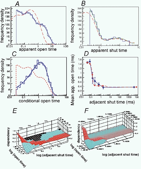
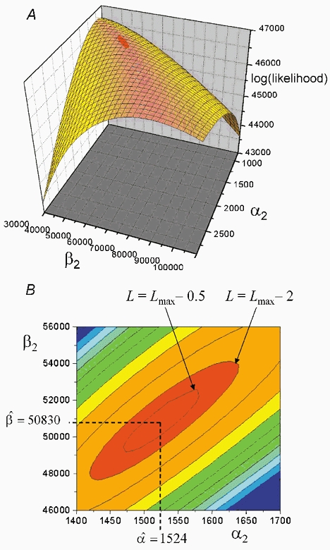
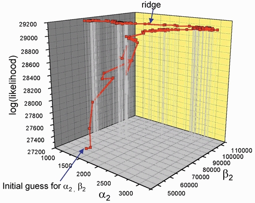
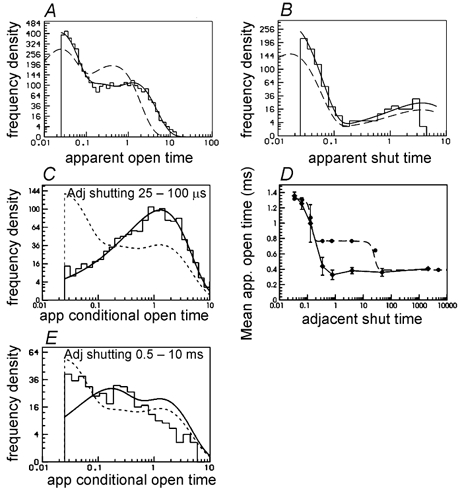
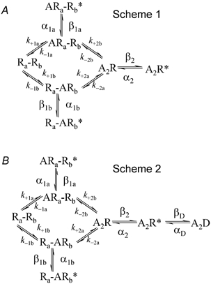
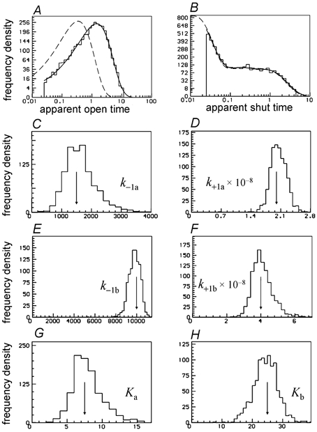
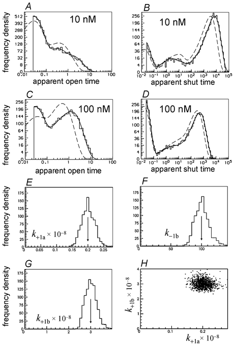
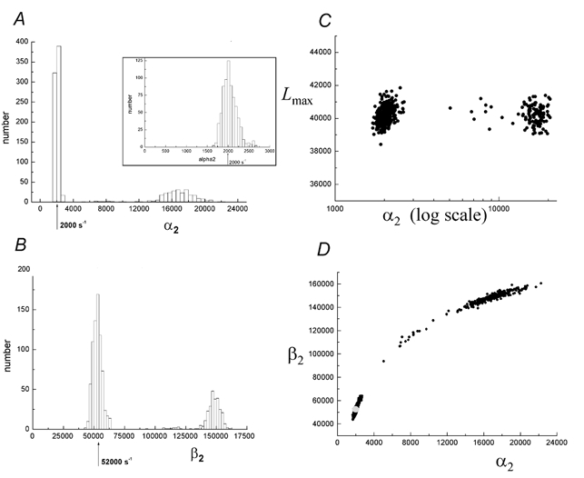
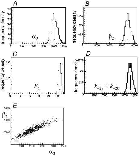
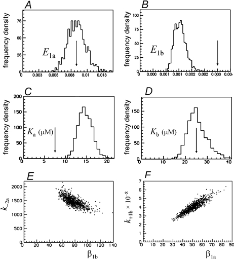
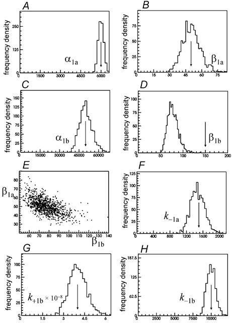
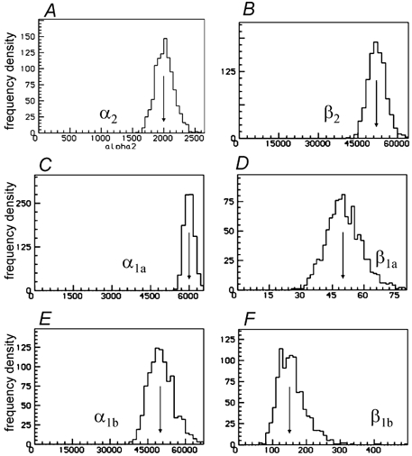
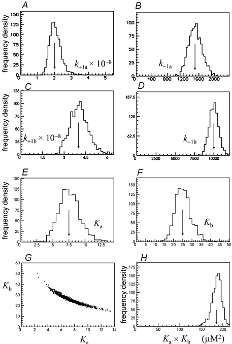
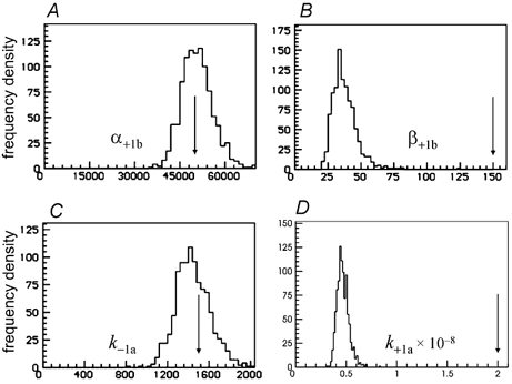
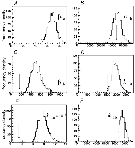
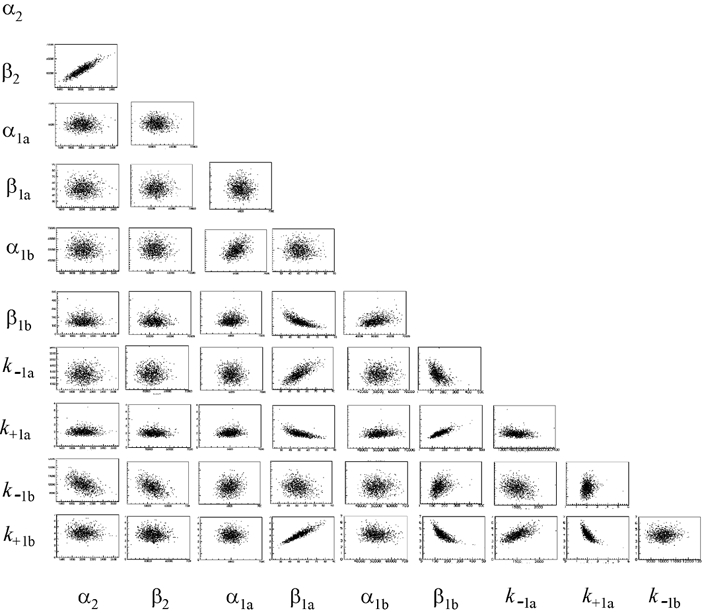
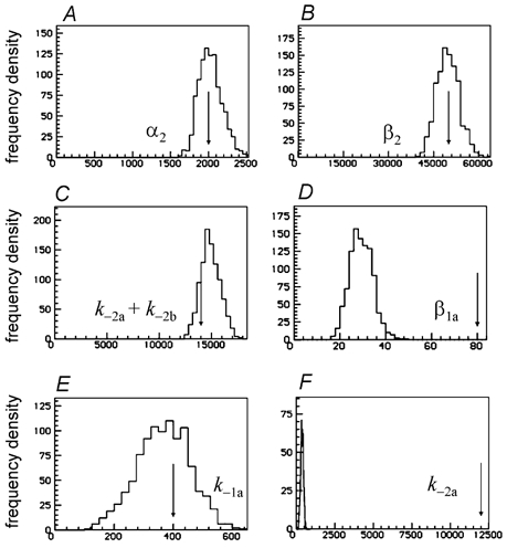
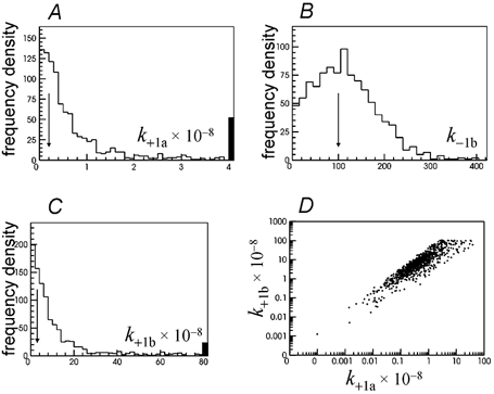
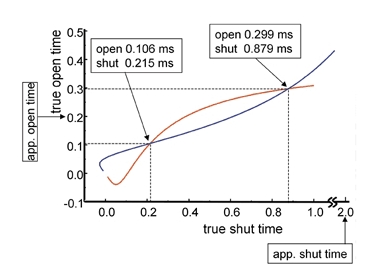
Properties of maximum likelihood estimators of rate constants for channel mechanisms are investigated, to see what can and cannot be inferred from experimental results. The implementation of the HJCFIT method is described; it maximises the likelihood of an entire sequence of apparent open and shut times, with the rate constants in a specified reaction mechanism as free parameters. The exact method for missed brief events is used. Several methods for testing the quality of the fit are described. The distributions of rate constants, and correlations between them, are investigated by doing sets of 1000 fits to simulated experiments. In a standard nicotinic receptor mechanism, all nine free rate constants can be estimated even from one single channel recording, as long as the two binding sites are independent, even when the number of channels in the patch is not known. The estimates of rate constants that apply to diliganded channels are robust; good estimates can be obtained even with erroneous assumptions (e.g. about the value of a fixed rate constant or the independence of sites). Rate constants that require distinction between the two sites are less robust, and require that an EC50 be specified, or that records at two concentrations be fitted simultaneously. Despite the complexity of the problem, it appears that there exist two solutions with very similar likelihoods, as in the simplest case. The hazards that result from this, and from the strong positive correlation between estimates of opening and shutting rates, are discussed.

Figure 6. Tests of the quality of the fit produced in a single simulated experiment of the same sort as the 1000 simulations used to generate Figs 3–5

A, histogram of distribution of apparent (‘observed’) open times with a resolution of 25 μs. The solid blue line shows the HJC open time distribution predicted by the fitted values of the rate constants with a resolution of 25 μs. Dashed red line: the open time distribution predicted by the fitted values of the rate constants without allowance for limited resolution - the estimate of the true open time distribution. B, as in A but for apparent shut times (note that only shut times up to t_crit= 3.5 ms are used for fitting so only these appear in the histogram). The HJC distribution is, as always, calculated from the exact expressions up to 3t_res (i.e. up to 75 μs in this case), and thereafter from the asymptotic form. Green line: the asymptotic form plotted right down to t_res= 25 μs. It is seen to become completely indistinguishable from the exact form for intervals above about 40 μs. C, histogram of distribution of ‘observed’ open times with a resolution of 25 μs for openings that are adjacent to short shuttings (durations between 25 and 100 μs). Solid line: the corresponding HJC conditional open time distribution predicted by the fitted values of the rate constants with a resolution of 25 μs. Dashed line: the HJC distribution of all open times (same as the solid line in A). D, conditional mean open time plot. The solid diamonds show the observed mean open time for apparent openings (resolution 25 μs) that are adjacent to apparent shut times in each of seven shut time ranges (plotted against the mean of these shut times). The bars show the standard deviations for each mean. The shut time ranges used were (ms) 0.025–0.05, 0.05–0.1, 0.1–0.2, 0.2–2, 2–20, 20–200 and > 200. Note, however, that shut time greater than t_crit (3.5 ms) will be shorter than predicted if there was more than one channel in the patch so the values on the abscissa above 3.5 ms are unreliable. The solid circles show the corresponding HJC conditional mean open times predicted by the fitted values of the rate constants with a resolution of 25 μs, for each of the seven ranges. The dashed line shows the continuous HJC relationship between apparent mean open times conditional on being adjacent to the shut time specified on the abscissa. E, ‘observed’ dependency plot for apparent open times and adjacent shut times (resolution 25 μs). Regions of positive correlation (dependency greater than zero) are red, negative correlations are blue, and black areas indicate regions where there were not enough observations to plot. F, fitted HJC dependency plot, predicted by the fitted values of the rate constants with a resolution of 25 μs.

Figure 12. The shape of the likelihood surface near its maximum

A, the surface shows the likelihood for various values of the shutting rate α₂, and the opening rate β₂, for the doubly occupied receptor. In order to plot this surface, the seven other free parameters were fixed at their maximum likelihood values, and the likelihood was calculated for various values of α₂ and β₂. B, contour representation of the surface shown in A, near the maximum. Dashed lines show the coordinates of the maximum point, the maximum likelihood estimates being α₂= 1524 s⁻¹ and β₂= 50 830 s⁻¹. The contours are shown also for log(likelihood) values of L=L_max− 0.5 and L=L_max− 2.0.

Figure 13. The progress of fitting in one example

The likelihood (vertical axis) that corresponds with the values of α₂ and β₂ that are reached at various stages during the fitting process - notice the final crawl along a diagonal ridge near the maximum. Along the ridge, the values of α₂ and β₂ change roughly in parallel (so the efficacy, E₂=β₂/α₂, does not change much), and the likelihood increases only slowly.

Figure 14. Predicted fits to a simulated experiment, when the fit assumed, incorrectly, that the two sites were independent

A single low concentration of ACh (30 nm) was used, with EC₅₀ constraint and fitted in bursts. The rate constants used for simulation are in Table 1 (labelled ‘true 2’), but the fit applied the constraints in eqns (9) and (10). A and B, predicted fits to apparent open and shut time, as in Fig. 6. C, conditional distribution of open times for apparent openings that are adjacent to the shortest shut times (25 - 100 μs). D, observed and predicted conditional mean open time plot (as in Fig. 6D and Methods). E, as in C but for apparent open times that are adjacent to shut times in the range 0.5–10 ms.

Figure 1. The two reaction schemes that were used for simulation of experiments

A = agonist, R = shut channel, R^*= open channel. R_a= the a binding site, R_b= the b binding site. D = desensitized channel.

Figure 16. Analysis of 1000 fits to simulated experiments at a single high (10 μm) concentration of ACh

The arrows mark the true values of the rate constants. A, apparent open times from a single simulated experiment, with the HJC distribution predicted by the fit superimposed on the histogram (resolution 25 μs); the dashed line is the predicted true distribution. B, apparent shut times (up to t_crit= 5 ms) as in A. C–F, distributions of 1000 estimates of the association and dissociation rate constants. G–H, distributions of the 1000 estimates of the microscopic equilibrium constants, K_a and K_b, for binding to the two sites (calculated from the fitted rate constants).

Figure 18. Non-independent sites

Illustration of the prediction of the distribution of apparent open and shut times by the rate constants estimated by a single simultaneous fit to two low concentration of ACh (10 nm and 100 nm) simulated experiments. In this case it was assumed that one channel was present throughout both records so the entire shut time distribution is fitted (B and D). The two sites were not assumed to be independent in this case, and good estimates were obtained for all 13 free rate constants (see text). In particular the three rate constants which could not be estimated when the number of channels was not assumed (Fig. 17A–C) are now estimated well (E–G), and the estimates of k_+1a and k_+1b are now essentially uncorrelated (H). The arrows mark the true values of the rate constants.

Figure 2. Distributions of the 1000 estimates of rate constants found by fitting, with HJCFIT, to 1000 simulated experiments

The arrows mark the true value of the rate constants. The simulation used the true rate constants given in Table 1 (‘true 1’), and each fit started from ‘guess 1’ (Table 1). Each ‘experiment’ consisted of 20 000 transitions (about 9000 transitions after the resolution of 25 μs was imposed), at a single low concentration, 30 nm, of ACh. The fitting was done in bursts of openings defined by a t_crit= 3.5 ms, with CHS vectors (see Methods). The sites were assumed to be independent (eqn (9)), and k_+1a=k_+2a was fixed at 1 × 10⁸m⁻¹ s⁻¹ (half its true value in this case). A, distribution of 1000 estimates of α₂. The inset shows the region near 2000 s⁻¹ enlarged. B, estimates of the 1000 estimates of β₂ from the same fits as used for A. C, the maximum likelihood (L_max) attained in each of the 1000 fits plotted against the value of α₂ from that fit D, the value of α₂ from each of the 1000 fits plotted against the value of β₂ from the same fit. The pale circle marks the true values.

Figure 3. Distribution of estimates of rate constants, and of quantities derived from them, for 1000 fits to experiments simulated as in Table 1 (starting from ‘guess 2’)

The arrows mark the true values of the rate constants. Each ‘experiment’ consisted of about 9000 transitions at a single low concentration, 30 nm, of ACh. The constraints in eqns (9) and (10) were true for the mechanism used for simulation, and were applied during the fit. In these fits k_+1a=k_+2a was fixed arbitrarily at 1 × 10⁸m⁻¹s⁻¹, half its true value. Distribution of 1000 estimates of A, α₂; B, β₂; C, E₂=β₂/α₂; D, k_−2a+k_−2b. The graph in E shows the 1000 pairs of α₂ and β₂ values plotted against each other to show the positive correlation between them (r=+0.916, see Table 3).

Figure 5. Distributions of equilibrium constants for the same fits as in Figs 3 and 4

A–D, distributions of the four equilibrium constants (E_1a, E_1b, K_a, K_b) that refer to the two separate sites, calculated from the fitted rate constants (as shown Figs 3 and 4). The arrows mark the true values of the rate constants. E, the negative correlation between k_−2a(=k_−1a) and β_1b; F, the positive correlation between k_+1b (=k_+2b) and β_1a.

Figure 4. Distributions of the ‘one site’ rate constants for the same set of 1000 fits as in Fig. 3

The arrows mark the true values of the rate constants.

Figure 7. The six gating rate constants

Single low concentration of ACh(30 nm) fitted in bursts (t_crit= 3.5 ms), with the two sites constrained to be independent. No parameters were fixed but k_+1a=k_+2a was calculated from the other rates so as to give the specified (correct) EC₅₀. The arrows mark the true values of the rate constants.

Figure 8. The same set of fits, with constrained EC₅₀, as shown in Fig. 7

A–D, distributions of the four binding rate constants, and E,F, two derived equilibrium constants, K_a and K_b. G, plot of K_b against K_a for each of the 1000 fits; H, distribution of the product K_aK_b. The arrows mark the true values of the rate constants.

Figure 9. Single low concentration of ACh (30 nm) fitted as in Figs 7 and 8, apart from specification of an incorrect value for the EC₅₀, twice its correct value

The arrows mark the true values of the rate constants.

Figure 10. Single low concentration of ACh (30 nm) fitted as in Figs 7 and 8, apart from specification of an incorrect value for the EC₅₀, half its correct value

The arrows mark the true values of the rate constants.

Figure 11. Correlation matrix shown graphically for the 1000 fits illustrated in Figs 7 and 8

Fitted values are plotted for the 45 possible pairs of parameters.

Figure 15. Distributions of some of the rate constant estimates obtained from 1000 fits under the same conditions as Fig. 14

The fits assumed, incorrectly, that the two sites were independent. The arrows mark the true values of the rate constants.

Figure 17. Non-independent sites

Estimates of k_+1a (A), k_−1b (B) and k_+1b (C) from 1000 simulated fits using simultaneous fit of three concentrations of ACh (10 nm, 30 nm and 100 nm), with a resolution of 10 μs. All three records were fitted in bursts (t_crit= 3.5 ms), using CHS vectors. D, plot of the estimate of k_+1b against that of k_+1a from the same fit (an upper limit of 10¹⁰m⁻¹ s⁻¹ was placed on association rate constants in these fits). The arrows mark the true values of the rate constants.

Figure 19. Two solutions for missed events problem in the simplest case

The two curves are plots of eqns (121) and (122) in Colquhoun & Hawkes (1995b, p. 456), for the example cited there in which the apparent mean open and shut times are 0.2 ms and 2.0 ms respectively, and the resolution was t_res= 0.2 ms. The intersections show that these simultaneous equations are satisfied either by true open and shut times of 0.299 and 0.879 ms respectively (the ‘slow solution’), and equally by true open and shut times of 0.106 and 0.215 ms respectively (the ‘fast solution’).

References

1. Akk G, Steinbach JH. Structural elements near the C-terminus are responsible for changes in nicotinic receptor gating kinetics following patch excision. J Physiol. 2000;527:405–417. - PMC - PubMed
1. Ball FG, Davies SS, Sansom MSP. Aggregated Markov processes incorporating time interval omission. Adv Appl Prob. 1988a;20:546–572.
1. Ball FG, Davies SS, Sansom MS. Single-channel data and missed events: analysis of a two-state Markov model. Proc R Soc Lond B Biol Sci. 1990;242:61–67. - PubMed
1. Ball FG, Sansom MSP. Single channel autocorrelation functions. The effects of time interval omission. Biophys J. 1988b;53:819–832. - PMC - PubMed
1. Ball FG, Sansom MSP. Ion channel gating mechanisms: model identification and parameter estimation from single channel recordings. Proc R Soc Lond B Biol Sci. 1989;236:385–416. - PubMed
Publication types
LinkOut - more resources