Azimuthal frustration and bundling in columnar DNA aggregates

Abstract

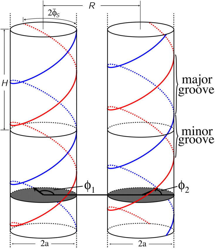
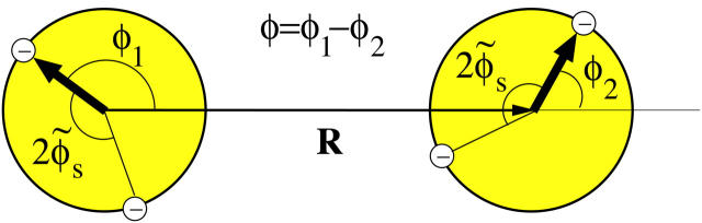
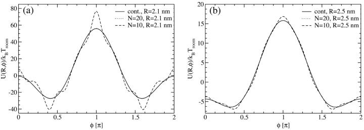
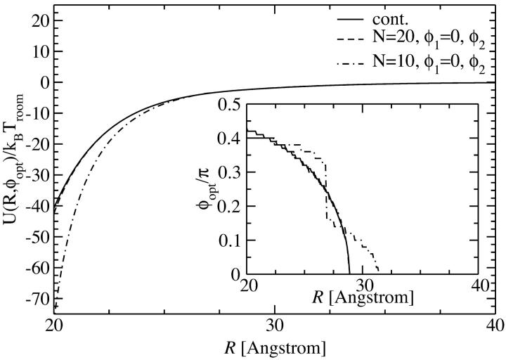
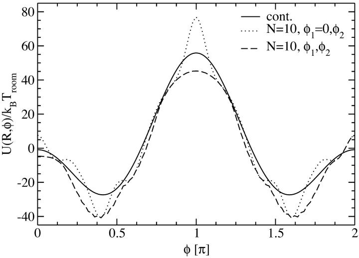
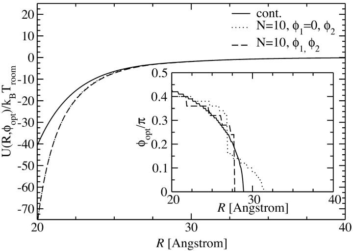
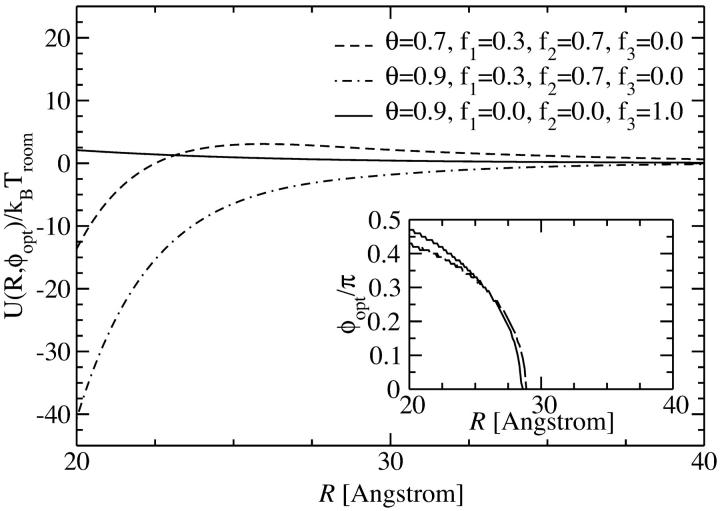
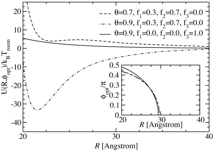
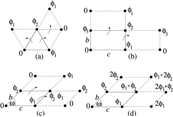
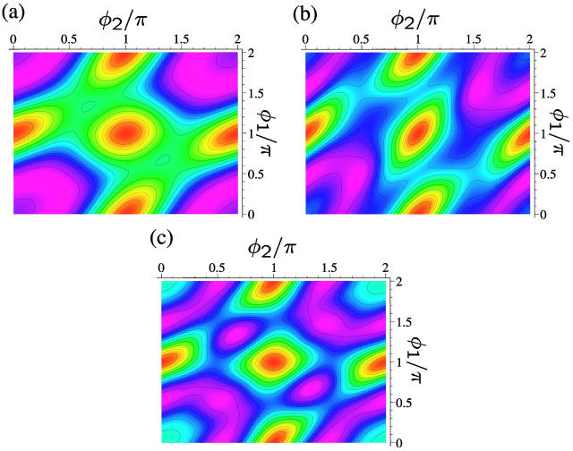
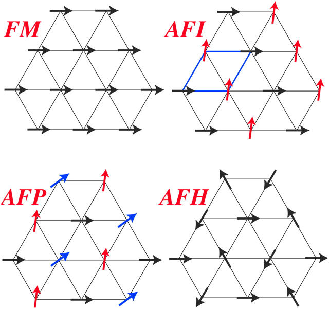
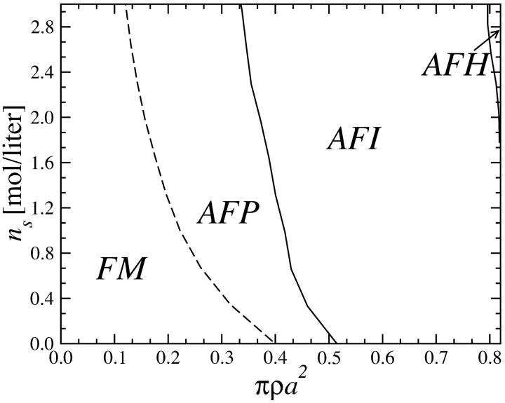
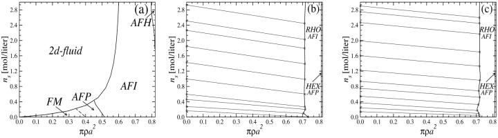
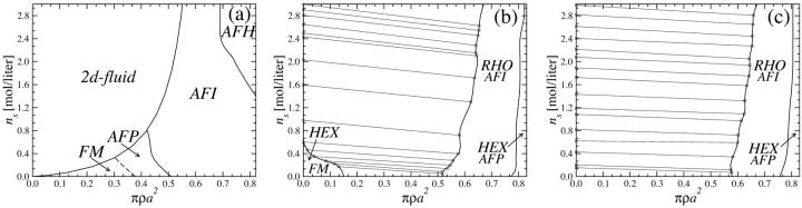
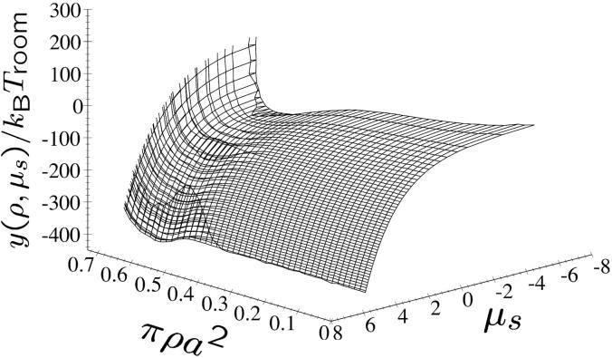
The interaction between two stiff parallel DNA molecules is discussed using linear Debye-Hückel screening theory with and without inclusion of the dielectric discontinuity at the DNA surface, taking into account the helical symmetry of DNA. The pair potential furthermore includes the amount and distribution of counterions adsorbed on the DNA surface. The interaction does not only depend on the interaxial separation of two DNA molecules, but also on their azimuthal orientation. The optimal mutual azimuthal angle is a function of the DNA-DNA interaxial separation, which leads to azimuthal frustrations in an aggregate. On the basis of the pair potential, the positional and orientational order in columnar B-DNA assemblies in solution is investigated. Phase diagrams are calculated using lattice sums supplemented with the entropic contributions of the counterions in solution. A variety of positionally and azimuthally ordered phases and bundling transitions is predicted, which strongly depend on the counterion adsorption patterns.

FIGURE 1

Illustration of two model DNA molecules at an interaxial separation R. The molecules are assumed to be rigid, long cylinders of radius a with a helical pitch length of H ≈ 34 Å. In between the two DNA helices a major and a minor groove are formed, due to the asymmetry in the azimuthal angle between the two helices, 2φ_s ≈ 0.8. See text and Fig. 2 for an explanation of the angles φ₁ and φ₂.

FIGURE 2

A plane perpendicular to the parallel axes of two DNA molecules separated by vector R hits the DNA strands denoted by the white circles with a minus inside; 2_s is the azimuthal width of the minor groove. The vectors joining the axes with the points where the 5′–3′ strand (Sinden, 1994) hits the plane may be formally called spins. The angle φ between the two spins characterizes the mutual azimuthal orientation of the molecules.

FIGURE 3

Yukawa-segment pair potential per length L_p as a function of the azimuthal orientation angle φ₂ with φ₁ = 0 fixed, at interaxial separations (a) R = 2.1 nm and (b) R = 2.5 nm, for θ = 0.9 and f₁ = 0.3, f₂ = 0.7, and f₃ = 0. At both interaxial separations the potential is displayed for N = 10, N = 20 charges as well as for continuous line charges.

FIGURE 4

Yukawa-segment pair potential per length L_p as a function of the interaxial separation R of two DNA molecules, at the optimal angle φ_2,opt(R), depicted for N = 10, N = 20 charges as well as for continuous line charges. The dependence of the optimal angle on the interaxial separation R is shown in the inset.

FIGURE 5

Yukawa-segment pair potential per length L_p as a function of the azimuthal orientation angle φ (solid line, continuous line charge distribution), as a function of φ = φ₁ − φ₂ with the optimal combination of φ₁ and φ₂ as described in the text (dashed line, N = 10 discrete charges) and as function of φ₂ with φ₁ = 0 fixed (dotted line, N = 10 discrete charges). All interactions are at an interaxial separation R = 2.1 nm, for θ = 0.9 and f₁ = 0.3, f₂ = 0.7, and f₃ = 0.

FIGURE 6

Yukawa-segment pair potential per length L_p as a function of the interaxial separation R of two DNA molecules, at the optimal azimuthal orientation angle φ_opt (solid line, continuous line charge distribution), at the optimal angle φ_opt = (φ₁ − φ₂)_opt with the optimal combination of φ₁ and φ₂, as described in the text (dashed line, N = 10 discrete charges) and as function of φ₂ with φ₁ = 0 fixed (dotted line, N = 10 discrete charges). All interactions are for counterion condensation parameters θ = 0.9 and f₁ = 0.3, f₂ = 0.7, and f₃ = 0. The dependence of the optimal angle on the interaxial separation R is shown in the inset.

FIGURE 7

Yukawa-segment pair potential for two segments of length L_p as a function of the mutual azimuthal orientation angle φ of two DNA molecules, at fixed interaxial separations as indicated in the legend, for θ = 0.9 and θ = 0.7. f₁=0.3, f₂ = 0.7, and f₃ = 0 were used for the fractions of condensed counterions in the minor and major groove and on the strands, at different interaxial separations, as indicated in the legend.

FIGURE 8

Yukawa-segment pair potential for two segments of length L_p as a function of the interaxial separation R of two DNA molecules, at the optimal angle φ_opt(R), depicted for different values of the counterion condensation parameter and for different counterion adsorption patterns. The dependence of the optimal angle on the interaxial separation R is shown in the inset.

FIGURE 9

Kornyshev-Leikin pair potential as a function of the interaxial separation R of two DNA molecules, at the optimal angle φ_opt(R), depicted for different values of the counterion condensation parameter and for different counterion adsorption patterns. The dependence of the optimal angle on the interaxial separation R is shown in the inset.

FIGURE 10

A schematic view of generating candidate ordered spin phases of the system. (a) for the HEX lattice; (b) for the REC and SQ lattices; and (c) and (d) for the RHO and OBL lattices.

FIGURE 11

Lines of constant energy as stemming from lattice sum calculations of DNA-salt mixtures for the KL model as a function of the azimuthal angles φ₁ and φ₂, with θ = 0.9 and f₁ = f₂ = 0, f₃ = 1. Magenta indicates low energies whereas red encodes high energy values. The lattice here is HEX. (a) πρa² = 0.44, n_s = 0.2 mol/l; (b) πρa² = 0.60, n_s = 0.2 mol/l; and (c) πρa² = 0.75, n_s = 1.7 mol/l.

FIGURE 12

The four stable magnetic phases. The arrows indicate the azimuthal orientations of DNA molecules. The acronyms, using magnetic terminology, stand for ferromagnetic (FM), antiferromagnetic Ising (AFI), antiferromagnetic Potts (AFP), and antiferromagnetic Heisenberg (AFH).

FIGURE 13

Phase diagram of DNA-salt mixtures for the YS model as a function of the DNA packing fraction πρa² and salt concentration n_s in the aggregate: θ = 0.9, f₁ = f₂ = 0, and f₃ = 1; the lattice here is HEX. Dashed lines denote second-order magnetic transitions, solid lines first-order ones.

FIGURE 14

Phase diagrams of DNA-salt mixtures for the YS model as a function of the DNA packing fraction πρa² and salt concentration n_s in the aggregate: (a) θ = 0.9, f₃ = 1; the lattice here is HEX. (b) θ = 0.7, f₁ = 0.3, and f₂ = 0.7; (c) θ = 0.9, f₁ = 0.3, and f₂ = 0.7. Dashed lines denote second-order magnetic transitions, solid lines first-order ones. The geometrical transitions between different lattices in b and c are second order; the straight lines are tielines between coexisting phases.

FIGURE 15

A possible SQ phase with orthogonal magnetic ordering.

FIGURE 16

Phase diagrams of DNA-salt mixtures for the KL model as a function of the DNA packing fraction πρa² and salt concentration n_s in the aggregate: (a) θ = 0.9, f₃ = 1; the lattice here is HEX. (b) θ = 0.7, f₁ = 0.3, and f₂ = 0.7; (c) θ = 0.9, f₁ = 0.3, and f₂ = 0.7. Dashed lines denote second-order magnetic transitions, solid lines first-order ones. The geometrical transitions between different lattices in b and c are second order; the straight lines are tielines between coexisting phases.

FIGURE 17

Semigrand potential per unit volume y(ρ,μ_s) as a function of reduced DNA density and salt chemical potential, for the KL model and parameters θ = 0.9, f₁ = 0.3, f₂ = 0.7, and f₃ = 0.

FIGURE 18

Semigrand potential per unit volume y(ρ,μ_s) on a line of constant DNA chemical potential for the KL model as a function of the reduced DNA density and for parameters θ = 0.9, f₁ = 0.3, f₂ = 0.7, and f₃ = 0. Also shown (dashed line) is the common tangent connecting the coexisting phase points.

References

1. Allahyarov, E., and H. Löwen. 2000. Effective interaction between helical biomolecules. Phys. Rev. E. 62:5542–5556. - PubMed
1. Ashcroft, N. W., and D. Stroud. 1978. Theory of the thermodynamics of simple liquid metals. Sol. State Phys. 33:1–81.
1. Bloomfield, V. A. 1996. DNA condensation. Curr. Opin. Struct. Biol. 6:334–341. - PubMed
1. Canessa, E., M. J. Grimson, and M. Silbert. 1988. Volume dependent forces in charge stabilized colloidal crystals. J. Mol. Phys. 64:1195–1201.
1. Denton, A. R. 1999. Effective interactions and volume energies in charge-stabilized colloidal suspensions. J. Phys.: Condens. Matter 11:10061–10071; 2000.
Publication types
LinkOut - more resources