

doi: 10.1073/pnas.0932745100.
Epub 2003 Jun 9.
Connectivity optimization and the positioning of cortical areas
Affiliations
- PMID: 12796510
- PMCID: PMC164691
- DOI: 10.1073/pnas.0932745100
Item in Clipboard
Connectivity optimization and the positioning of cortical areas
Proc Natl Acad Sci U S A.
.
Abstract
By examining many alternative arrangements of cortical areas, we have found that the arrangement actually present in the brain minimizes the volume of the axons required for interconnecting the areas. Our observations support the notion that the organization of cortical areas has evolved to optimize interareal connections.
Figures

Identification of prefrontal cortical areas. (Inset) Lateral view of macaque cerebral cortex showing the general location of prefrontal cortical areas. (A) Ventromedial view of the right macaque cerebral cortex with the areas of the prefrontal cortex identified in color (10). The 11 selected areas (see text for details) are shown in colors other than yellow. Borders are also shown for some of the adjacent cortical areas identified in Carmichael and Price (10) that were not included in our calculations. (B) The same view as in A of the inflated cortex. This map and its flattened version were used to determine the surface-based coordinates of the area centers. Area color assignment is the same as in A and Inset.
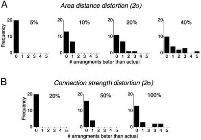
Robustness of connectivity optimization. A set of random, Gaussian-distributed numbers [with a mean of 0, and various SDs (σ), see Methods for details] was added to the matrix of interareal distances or to the matrix of connection weights. For each σ, 20 different randomly perturbed sets of areal positions or connection strengths were generated, and all possible permutations within the small and large area groups (this set of permutations is identical to that described in Fig. 3A) were examined. The frequency of appearance of arrangements better than control was plotted for distances (A) and for connection strengths (B) for each σ examined [2σ is shown above each plot as a percent of the average interareal distance (A) or connection strength (B)].
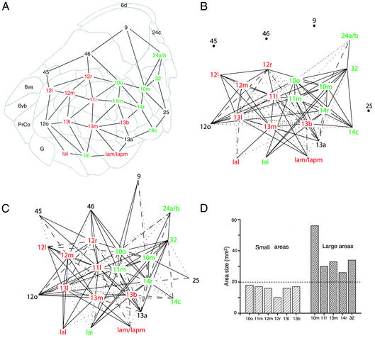
Connectivity between prefrontal cortical areas. (A) A map of the inflated prefrontal cortex (same view as in Fig. 1B) with 10 areas of the medial network identified in red and 8 areas of the orbital network identified in green. Other cortical areas that are not a part of the orbital–medial network are shown in black. The edges connect the areas of the prefrontal cortex that share a common border and appear in the connection matrix (see text for details). (B and C) The connection matrix for connections from B and to C for the 11 selected areas. From and to matrices contain 125 and 145 connections, respectively. The strength of connection, ranked from 0 (no connection) to 3 (strongest connection), is shown as follows: 0, no line; 1, dotted line; 2, dashed line; and 3, solid line. (D) A histogram of selected area sizes as determined from the control (uniflated) cortex. The selected areas were subdivided according to the histogram into two size groups: six small areas (<20 mm2) and five large areas (>20 mm2).
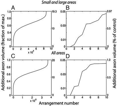
Additional axonal volume in alternative cortical configurations. Additional interareal axonal volume (compared with the axonal volume for the actual cortex) for all possible arrangements was ranked in ascending order and plotted versus its rank. Scales on the left are normalized and scales on the right give the percent change from actual cortex. (A) Six small and five large areas were permuted within each group and all possible combinations were considered for a total of 6!·5! = 86,400 alternative configurations. (B) Ten best configurations from A. The best configuration has 0 additional axonal volume and corresponds to the actual arrangement of areas. The second-best and third-best alternatives correspond to the exchange of areas 10m ↔ 32 and 10o ↔ 11m, respectively. In the worst alternative, all areas were misplaced from their positions. (C and D) Same as A and B, respectively, for all selected areas except for 10m. All possible permutations of 10 areas give 10! = 3.629 million alternative configurations. As in A, C shows the best configuration has 0 additional axonal volume and corresponds to the areal configuration of the actual cortex. Because area 10m is not moved in this calculation, the second-best alternative corresponds to the third best of A and B: exchange of areas 10o ↔ 11m. Third-best and fourth-best alternatives correspond to exchange of areas 11m ↔ 14r and 12m ↔ 13l, respectively. As in A, C shows that in the worst alternative configuration all areas were misplaced from their positions.
References
MeSH terms
LinkOut - more resources
Full Text Sources
