A population threshold for functional polymorphisms

Abstract

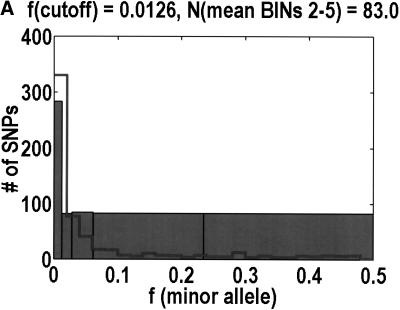
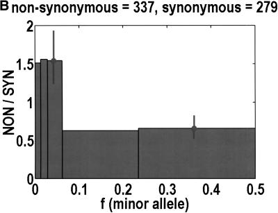
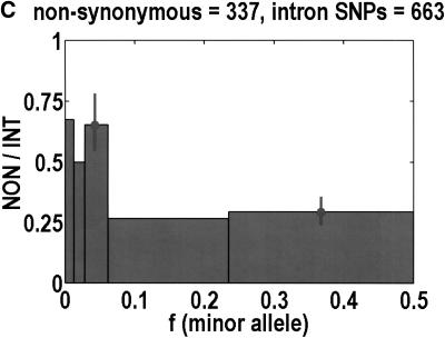
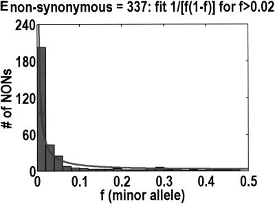
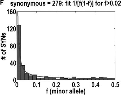
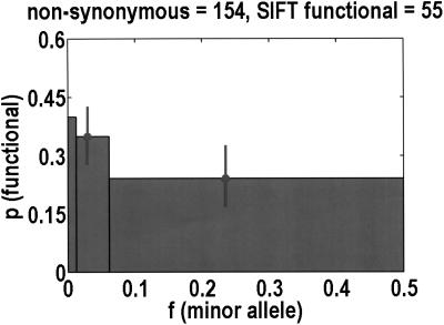
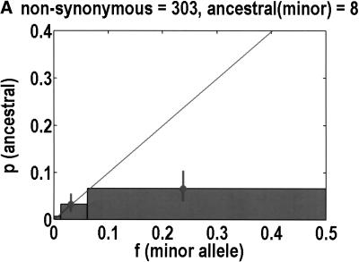
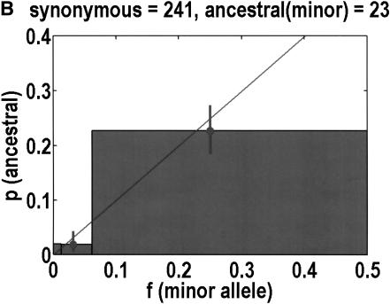
We sequenced 114 genes (for DNA repair, cell cycle arrest, apoptosis, and detoxification)in a mixed human population and observed a sudden increase in the number of functional polymorphisms below a minor allele frequency of approximately 6%. Functionality is assessed by considering the ratio in the number of nonsynonymous single nucletide polymorphisms (SNPs)to the number of synonymous or intron SNPs. This ratio is steady from below 1% in frequency-that regime traditionally associated with rare Mendelian diseases-all the way up to about 6% in frequency, after which it falls precipitously. We consider possible explanations for this threshold effect. There are four candidates as follows: (1). deleterious variants that have yet to be purified from the population, (2). balancing selection, in which a selective advantage accrues to the heterozygotes, (3). population-specific functional polymorphisms, and (4). adaptive variants that are accumulating in the population as a response to the dramatic environmental changes of the last 7000 approximately 17000 years.

Figure 1

To analyze ratios for the number of SNPs that are deemed nonsynonymous (NON), synonymous (SYN), and intron (INT), we partition the frequency axes into 5 nonuniform bins with boundaries 0.0000, 0.0126, 0.0280, 0.0614, 0.2346, and 0.5000. There are 284 coding SNPs in bin 1, and there is a mean of 83.0 coding SNPs in each of the bins 2–5. These panels depict (A) the number of coding SNPs, with a solid line for the same data plotted on a uniform bin size of 0.02, (B) the NON/SYN ratio, (C) the NON/INT ratio, and (D) the SYN/INT ratio. Error bars indicate standard deviation, assuming the data are sampled from a binomial distribution. All of the uncertainty is in bins 2–5. Error bars for bin 1 are much smaller and not indicated. The generally lower quality of the intron data is responsible for the glitch in bin 2 of panels C and D. At top of each panel, we indicate the number of SNPs in the stated categories. Finally, we demonstrate the futility of trying to make sense of these data by more conventional methods. Using a uniform bin size of 0.02, we plot the number of (E) NON and (F) SYN polymorphisms, and compare them with the neutral theory expectation of 1/[f(1-f)]. Our curve fitting procedures ignore the first bin to avoid the singlets and sampling uncertainties. Extrapolation of the curve fit back to the first bin is indicated by a filled circle. Only if one squints hard enough at the fit deviations, might one notice a change in NON/SYN ratio.

Figure 1

To analyze ratios for the number of SNPs that are deemed nonsynonymous (NON), synonymous (SYN), and intron (INT), we partition the frequency axes into 5 nonuniform bins with boundaries 0.0000, 0.0126, 0.0280, 0.0614, 0.2346, and 0.5000. There are 284 coding SNPs in bin 1, and there is a mean of 83.0 coding SNPs in each of the bins 2–5. These panels depict (A) the number of coding SNPs, with a solid line for the same data plotted on a uniform bin size of 0.02, (B) the NON/SYN ratio, (C) the NON/INT ratio, and (D) the SYN/INT ratio. Error bars indicate standard deviation, assuming the data are sampled from a binomial distribution. All of the uncertainty is in bins 2–5. Error bars for bin 1 are much smaller and not indicated. The generally lower quality of the intron data is responsible for the glitch in bin 2 of panels C and D. At top of each panel, we indicate the number of SNPs in the stated categories. Finally, we demonstrate the futility of trying to make sense of these data by more conventional methods. Using a uniform bin size of 0.02, we plot the number of (E) NON and (F) SYN polymorphisms, and compare them with the neutral theory expectation of 1/[f(1-f)]. Our curve fitting procedures ignore the first bin to avoid the singlets and sampling uncertainties. Extrapolation of the curve fit back to the first bin is indicated by a filled circle. Only if one squints hard enough at the fit deviations, might one notice a change in NON/SYN ratio.

Figure 1

To analyze ratios for the number of SNPs that are deemed nonsynonymous (NON), synonymous (SYN), and intron (INT), we partition the frequency axes into 5 nonuniform bins with boundaries 0.0000, 0.0126, 0.0280, 0.0614, 0.2346, and 0.5000. There are 284 coding SNPs in bin 1, and there is a mean of 83.0 coding SNPs in each of the bins 2–5. These panels depict (A) the number of coding SNPs, with a solid line for the same data plotted on a uniform bin size of 0.02, (B) the NON/SYN ratio, (C) the NON/INT ratio, and (D) the SYN/INT ratio. Error bars indicate standard deviation, assuming the data are sampled from a binomial distribution. All of the uncertainty is in bins 2–5. Error bars for bin 1 are much smaller and not indicated. The generally lower quality of the intron data is responsible for the glitch in bin 2 of panels C and D. At top of each panel, we indicate the number of SNPs in the stated categories. Finally, we demonstrate the futility of trying to make sense of these data by more conventional methods. Using a uniform bin size of 0.02, we plot the number of (E) NON and (F) SYN polymorphisms, and compare them with the neutral theory expectation of 1/[f(1-f)]. Our curve fitting procedures ignore the first bin to avoid the singlets and sampling uncertainties. Extrapolation of the curve fit back to the first bin is indicated by a filled circle. Only if one squints hard enough at the fit deviations, might one notice a change in NON/SYN ratio.

Figure 1

To analyze ratios for the number of SNPs that are deemed nonsynonymous (NON), synonymous (SYN), and intron (INT), we partition the frequency axes into 5 nonuniform bins with boundaries 0.0000, 0.0126, 0.0280, 0.0614, 0.2346, and 0.5000. There are 284 coding SNPs in bin 1, and there is a mean of 83.0 coding SNPs in each of the bins 2–5. These panels depict (A) the number of coding SNPs, with a solid line for the same data plotted on a uniform bin size of 0.02, (B) the NON/SYN ratio, (C) the NON/INT ratio, and (D) the SYN/INT ratio. Error bars indicate standard deviation, assuming the data are sampled from a binomial distribution. All of the uncertainty is in bins 2–5. Error bars for bin 1 are much smaller and not indicated. The generally lower quality of the intron data is responsible for the glitch in bin 2 of panels C and D. At top of each panel, we indicate the number of SNPs in the stated categories. Finally, we demonstrate the futility of trying to make sense of these data by more conventional methods. Using a uniform bin size of 0.02, we plot the number of (E) NON and (F) SYN polymorphisms, and compare them with the neutral theory expectation of 1/[f(1-f)]. Our curve fitting procedures ignore the first bin to avoid the singlets and sampling uncertainties. Extrapolation of the curve fit back to the first bin is indicated by a filled circle. Only if one squints hard enough at the fit deviations, might one notice a change in NON/SYN ratio.

Figure 1

To analyze ratios for the number of SNPs that are deemed nonsynonymous (NON), synonymous (SYN), and intron (INT), we partition the frequency axes into 5 nonuniform bins with boundaries 0.0000, 0.0126, 0.0280, 0.0614, 0.2346, and 0.5000. There are 284 coding SNPs in bin 1, and there is a mean of 83.0 coding SNPs in each of the bins 2–5. These panels depict (A) the number of coding SNPs, with a solid line for the same data plotted on a uniform bin size of 0.02, (B) the NON/SYN ratio, (C) the NON/INT ratio, and (D) the SYN/INT ratio. Error bars indicate standard deviation, assuming the data are sampled from a binomial distribution. All of the uncertainty is in bins 2–5. Error bars for bin 1 are much smaller and not indicated. The generally lower quality of the intron data is responsible for the glitch in bin 2 of panels C and D. At top of each panel, we indicate the number of SNPs in the stated categories. Finally, we demonstrate the futility of trying to make sense of these data by more conventional methods. Using a uniform bin size of 0.02, we plot the number of (E) NON and (F) SYN polymorphisms, and compare them with the neutral theory expectation of 1/[f(1-f)]. Our curve fitting procedures ignore the first bin to avoid the singlets and sampling uncertainties. Extrapolation of the curve fit back to the first bin is indicated by a filled circle. Only if one squints hard enough at the fit deviations, might one notice a change in NON/SYN ratio.

Figure 1

To analyze ratios for the number of SNPs that are deemed nonsynonymous (NON), synonymous (SYN), and intron (INT), we partition the frequency axes into 5 nonuniform bins with boundaries 0.0000, 0.0126, 0.0280, 0.0614, 0.2346, and 0.5000. There are 284 coding SNPs in bin 1, and there is a mean of 83.0 coding SNPs in each of the bins 2–5. These panels depict (A) the number of coding SNPs, with a solid line for the same data plotted on a uniform bin size of 0.02, (B) the NON/SYN ratio, (C) the NON/INT ratio, and (D) the SYN/INT ratio. Error bars indicate standard deviation, assuming the data are sampled from a binomial distribution. All of the uncertainty is in bins 2–5. Error bars for bin 1 are much smaller and not indicated. The generally lower quality of the intron data is responsible for the glitch in bin 2 of panels C and D. At top of each panel, we indicate the number of SNPs in the stated categories. Finally, we demonstrate the futility of trying to make sense of these data by more conventional methods. Using a uniform bin size of 0.02, we plot the number of (E) NON and (F) SYN polymorphisms, and compare them with the neutral theory expectation of 1/[f(1-f)]. Our curve fitting procedures ignore the first bin to avoid the singlets and sampling uncertainties. Extrapolation of the curve fit back to the first bin is indicated by a filled circle. Only if one squints hard enough at the fit deviations, might one notice a change in NON/SYN ratio.

Figure 2

The probability that a nonsynonymous SNP is functional is computed with the program SIFT, which considers the extent to which any polymorphic site is evolutionarily conserved across all good homologs in the public databases. Because only half of the nonsynonymous SNPs are SIFT analyzable, bin 1 is unchanged from Fig. 1, but bins 2 + 3 and 4 + 5 are merged together to improve statistics. Of these 154 analyzed SNPs, only 55 are predicted to be functional.

Figure 3

Ancestral alleles are determined by sequencing a chimpanzee and gorilla. We depict the probability that the minor allele is the ancestral allele. Bin 1 is unchanged from Fig. 1, but bins 2 + 3 and 4 + 5 are merged together to improve statistics. For each bin, we show the mean frequency as a filled circle. Data are divided into (A) nonsynonymous and (B) synonymous SNPs. Neutral theory predicts a straight line with a slope of 1, but this is observed only for synonymous SNPs.

Figure 3

Ancestral alleles are determined by sequencing a chimpanzee and gorilla. We depict the probability that the minor allele is the ancestral allele. Bin 1 is unchanged from Fig. 1, but bins 2 + 3 and 4 + 5 are merged together to improve statistics. For each bin, we show the mean frequency as a filled circle. Data are divided into (A) nonsynonymous and (B) synonymous SNPs. Neutral theory predicts a straight line with a slope of 1, but this is observed only for synonymous SNPs.

Figure 4

Growth in the frequency of the favored allele per generation, with dominant (D) and recessive (R) modes of inheritance. Predicted behavior is given for a range of linear selection coefficients s. Allele frequency for time zero is fixed at f0 = 0.010. The recessive mode behavior is sensitive to f0, in that it affects when the rapid transition from 0.1 to 0.9 can occur. Regardless of settings, this transition is always fast, relative to the asymptotic behavior at one or the other end.

References

1. Bailey, J.A., Gu, Z., Clark, R.A., Reinert, K., Samonte, R.V., Schwartz, S., Adams, M.D., Myers, E.W., Li, P.W., and Eichler, E.E. 2002. Recent segmental duplications in the human genome. Science 297: 1003-1007. - PubMed
1. Barbujani, G., Magagni, A., Minch, E., and Cavalli-Sforza, L.L. 1997. An apportionment of human DNA diversity. Proc. Natl. Acad. Sci. 94: 4516-4519. - PMC - PubMed
1. Bustamante, C.D., Wakeley, J., Sawyer, S., and Hartl, D.L. 2001. Directional selection and the site-frequency spectrum. Genetics 159: 1779-1788. - PMC - PubMed
1. Cargill, M., Altshuler, D., Ireland, J., Sklar, P., Ardlie, K., Patil, N., Shaw, N., Lane, C.R., Lim, E.P., Kalyanaraman, N., et al. 1999. Characterization of single-nucleotide polymorphisms in coding regions of human genes. Nat. Genet. 22: 231-238. - PubMed
1. Collins, F.S., Brooks, L.D., and Chakravarti, A. 1998. A DNA polymorphism discovery resource for research on human genetic variation. Genome Res. 8: 1229-1231. - PubMed
WEB SITE REFERENCES
1. http://www.genome.washington.edu/projects/egpsnps; University of Washington Genome Center Repository of Candidate-Gene Polymorphisms for Environmental Genome Project (EGP).
Publication types
MeSH terms
LinkOut - more resources