. 2003 Aug 20;23(20):7690-701.
doi: 10.1523/JNEUROSCI.23-20-07690.2003.

Time course and time-distance relationships for surround suppression in macaque V1 neurons

Affiliations

Time course and time-distance relationships for surround suppression in macaque V1 neurons

Wyeth Bair et al. J Neurosci. .

Abstract

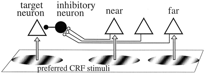
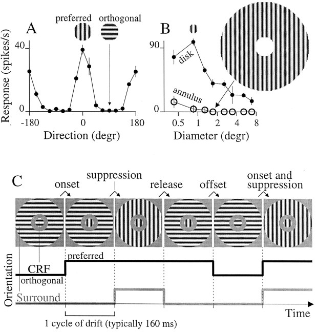
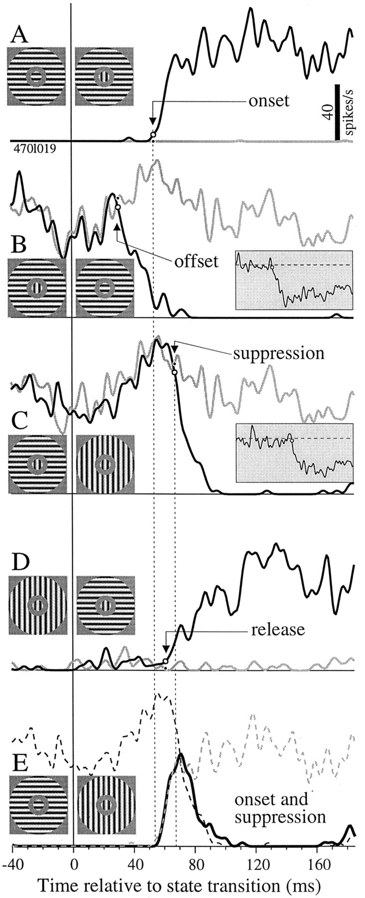
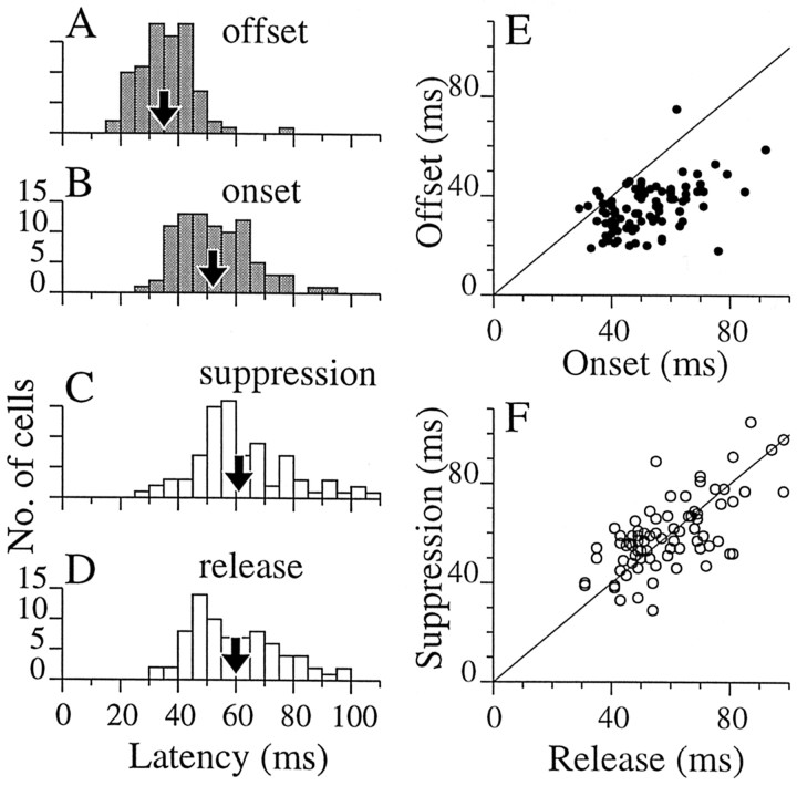
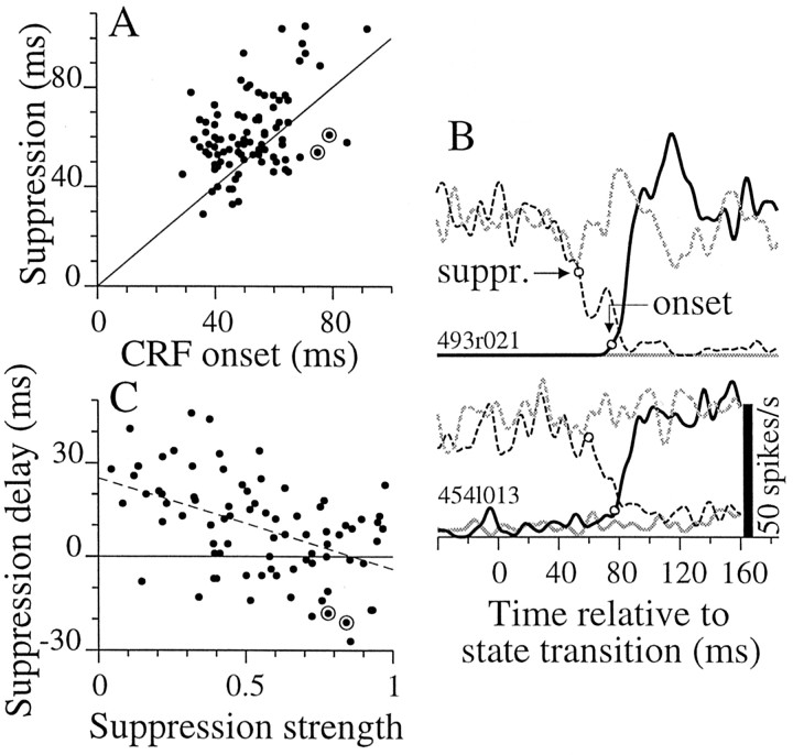
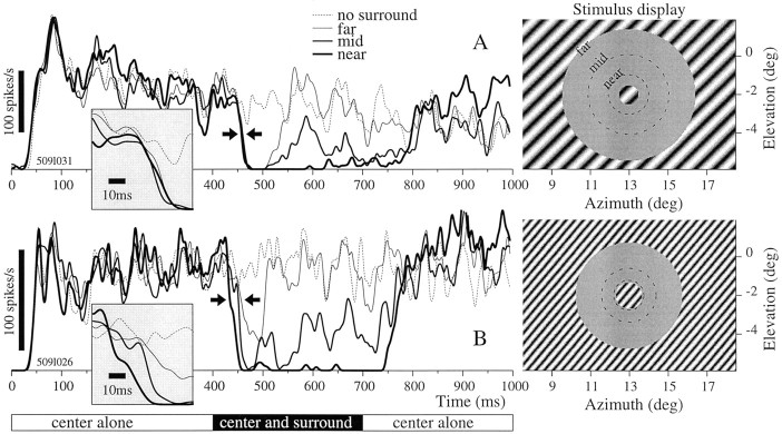
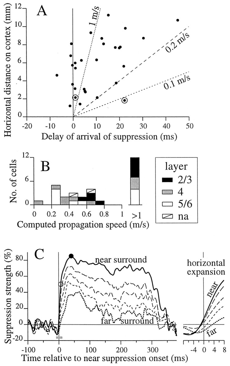
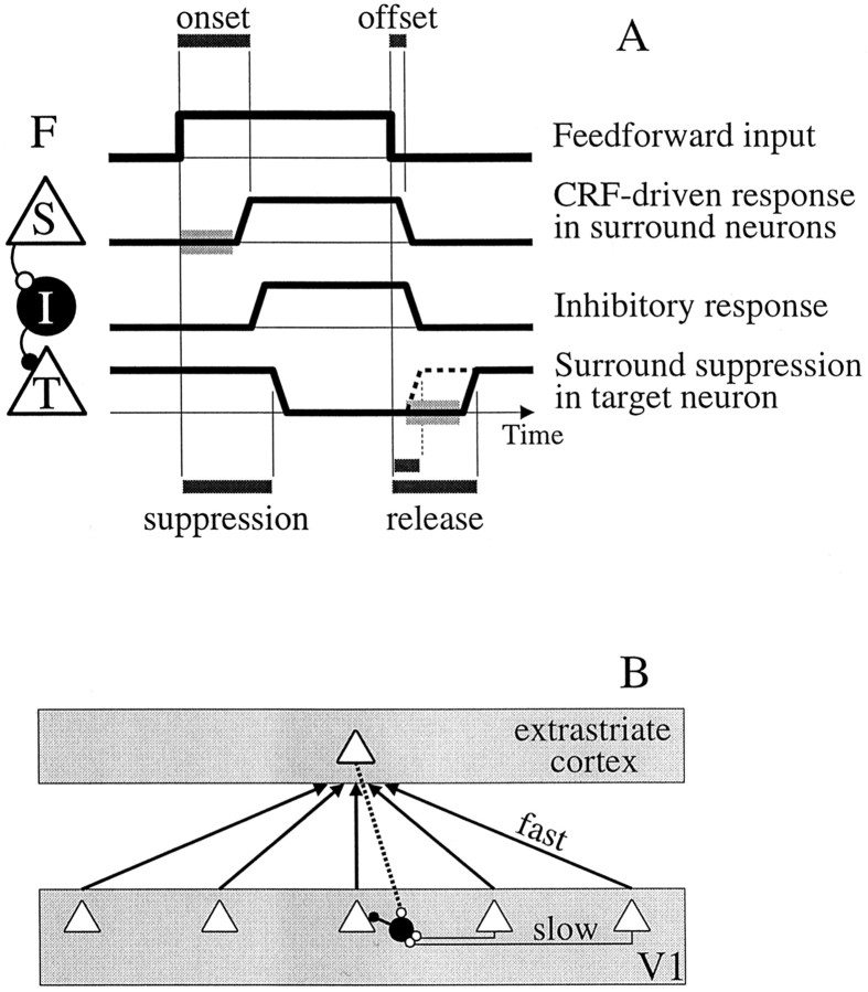
Iso-orientation surround suppression is a powerful form of visual contextual modulation in which a stimulus of the preferred orientation of a neuron placed outside the classical receptive field (CRF) of the neuron suppresses the response to stimuli within the CRF. This suppression is most often attributed to orientation-tuned signals that propagate laterally across the cortex, activating local inhibition. By studying the temporal properties of surround suppression, we have uncovered characteristics that challenge standard notions of surround suppression. We found that the latency of suppression depended on its strength. Across cells, strong suppression arrived on average 30 msec earlier than weak suppression, and suppression sometimes arrived faster than the excitatory CRF response. We compared the relative latency of CRF response onset and offset with the relative latency of suppression onset and offset. Response onset was delayed relative to response offset in the CRF but not in the surround. This is not the expected result if neurons targeted by suppression are like those that generate it. We examined the time course of suppression as a function of distance of the surround stimulus from the CRF and found that suppression was predominantly sustained for nearby stimuli and predominantly transient for distant stimuli. By comparing the latency of suppression for nearby and distant stimuli, we found that orientation-tuned suppression could effectively propagate across 6 - 8 mm of cortex at approximately 1 m/sec. This is considerably faster than expected for horizontal cortical connections previously implicated in surround suppression. We offer refinements to circuits for surround suppression that account for these results and describe how feedback from cells with large CRFs can account for the rapid propagation of suppression within V1.


Figures

Figure 1.
Figure 1.
Putative circuit for iso-orientation surround suppression in V1. The target neuron (left triangle) receives inhibition from a nearby neuron (large filled circle) that is driven by excitatory neurons displaced laterally in cortex (3 triangles at right) that have orientation tuning similar to the target cell. Preferred stimuli confined to the CRFs for three excitatory neurons are indicated by the circular patches of sinusoidal grating shown on the tilted plane that represents a two-dimensional visual field. Arrows emanating from the stimuli indicate localized feedforward inputs to the excitatory neurons. We find that this circuit is insufficient to account for some temporal features of surround suppression.
Figure 2.
Figure 2.
Tuning curves for orientation and size were used to configure our dynamic center-surround stimulus. A, The mean firing rate of an example neuron (3 trials, 4 sec/trial) is plotted against the drift direction (in degrees, relative to preferred) of a sinusoidal grating. Motion was always orthogonal to the orientation of the grating; therefore, we refer to this as an orientation tuning curve. Error bars indicate SEM. The stimulus of preferred orientation is shown by the icon above the peak at zero. The spontaneous rate for this neuron was zero. B, A size tuning curve (filled circles) shows mean response versus stimulus diameter for the same neuron. The optimal size (small icon) was smaller than that in A, which accounts for larger responses here. The annulus tuning curve (open circles) shows the response to gratings presented in an annular window versus the inner diameter of the annulus. The outer diameter was set to fill our screen. The CRF region (small icon) was the disk that optimized the size tuning curve. The surround region (large icon) was the annulus with the smallest inner diameter that did not elicit a response above the spontaneous firing rate. The arrow marks the inner diameter for the surround region. Icons here and in A are drawn to scale. C, The icons depict a succession of six states of the dynamic center-surround stimulus (see Materials and Methods). The gratings in the CRF (center disk) and surround (annulus) drifted in either the preferred direction (shown as vertical) or in an orthogonal direction (horizontal). For clarity, the surround annulus outer diameter is shown here at 50% of the size determined in B. Below the icons, orientation is plotted versus time for the CRF (black line) and surround (gray line). The state transitions of interest here are labeled above the bent arrows. This sequence was chosen for convenient demonstration; the actual sequence of transitions was random.
Figure 3.
Figure 3.
The dynamic center-surround stimulus elicited rapid increases and decreases in firing rate via the CRF and the surround. In each plot, the black trace shows the mean firing rate (calibration in A) versus time for the stimulus transition indicated by the pair of icons. The icons straddle t = 0, the time of the stimulus transition. A-D, Reference curves (gray lines) show the response to two consecutive periods of the stimulus indicated by the left icon. All curves are averages over 100-120 repeats (see Materials and Methods). A, The response increased when the CRF stimulus changed from orthogonal (shown as horizontal in icons) to preferred (vertical) but the surround orientation stayed orthogonal (nonsuppressive). The reference response, ∼0 spikes/sec, lies on the x-axis. The arrow labeled onset points to an open circle on the response curve (black line) and shows the response latency, which is defined as the time of 5% rise to the maximum difference between the response and the reference curves (see Materials and Methods). The distance from the open circle to the black dot (on the reference curve) indicates the 5% response difference. The onset time is also marked by a vertical dotted line for comparison with plots below. B, The response decreased when the CRF stimulus changed from preferred to orthogonal (with orthogonal surround). This response offset began earlier (arrow) than the response onset in A. The inset shows the difference between the response and reference curves, where the dashed line is 0 difference, and the circle marks 5% of the maximum difference. C, The response to the preferred CRF stimulus was suppressed by a transition of the surround from orthogonal to preferred. The decrease was at least as rapid as that for CRF offset in B. Suppression latency (arrow) is indicated by a vertical dotted line. The inset shows the difference, as in B. D, The release of suppression, caused by the surround changing to orthogonal with the CRF stimulus remaining preferred, occurred at about the same time (arrow) as suppression in C. E, A simultaneous change in the center and the surround caused a response (thick line) that followed the CRF onset response (gray dashed line, replotted from A) until approximately the time of suppression (right vertical dotted line). Thereafter, the response followed the time course of suppression (black dashed line, replotted from C).
Figure 4.
Figure 4.
Comparison of response timing for CRF and surround signals across cells. A-D, The distribution of response latencies (see Materials and Methods) for CRF transitions (gray histograms) and surround transitions (open histograms) are plotted for 92 cells (arrows show means). On average, CRF offset (A) was earliest (35 msec; SD, 10 msec). CRF onset (B) occurred on average 17 msec later (52 msec; SD, 13 msec). Surround modulation occurred the latest on average [61 and 60 msec for suppression (C) and release (D), respectively; SD, 17 msec]. E, For each neuron, offset time is plotted against onset time. Almost all points fall below the unity diagonal, indicating that almost all cells responded to the offset faster than to the onset of the preferred stimulus in the CRF. Offset latency also was significantly less variable than onset latency (SD, 9.7 and 13 msec; F test, p = 0.009). F, For the surround, suppression time is plotted against release time. These values were on average not different across cells (paired t test, p = 0.87; n = 85) and were significantly correlated (r = 0.70; p < 10-6).
Figure 5.
Figure 5.
Latency of suppression relative to CRF onset. A, Suppression latency is plotted against CRF onset latency for 87 cells. In most cells, suppression arrived later than CRF excitation, but in some (points below diagonal line), suppression arrived sooner. B, For two example cells (A, C, circled points) for which suppression came before onset, response curves are shown for suppression (suppr.; dashed lines) and onset (solid lines). Solid lines show response (black) and reference (gray) curves for the transition like that of Fig. 3A. Dashed lines show the response (black) and reference (gray) curves for the transition like that of Fig. 3C. Open circles mark 5% latencies, as in A and C. C, For each cell, suppression delay (suppression latency minus CRF onset latency) is plotted against suppression strength (1 indicates complete suppression; 0, no suppression). There is a significant negative correlation between suppression delay and strength (r = -0.48; p < 10-5; n = 87). Strong suppression often occurred as early as CRF onset, whereas weak suppression was delayed by ∼30 msec on average. The dashed line shows a linear regression.
Figure 6.
Figure 6.
The time course of suppression is shown for surround stimuli that lie at several distances from the CRF for two example neurons. A, The stimulus display (right) shows the CRF stimulus, which was a central patch of grating optimized for the CRF, and the far surround stimulus, which was a grating extending from the edges of the display to a circular inner border. The dashed circles mark inner borders for two other surround stimuli: the mid and near surrounds. The CRF stimulus appeared for 1 sec starting at t = 0, and the surround stimulus appeared for 300 msec starting at t = 400 msec (timing bar at bottom). The preferred orientation and spatial frequency were as shown. The mean firing rates (n = 20 trials, convolved with Gaussian; SD, 4 msec) are shown for the near, mid, and far surrounds (thick to thin lines). The response to the CRF stimulus alone is shown by the dotted line. The near surround strongly suppressed the response to the CRF (thickest black line; arrows indicate onset of suppression). The suppression caused by the mid surround initially had a time course similar to that of the far surround but became weaker after ∼50 msec. The far surround suppression (thin solid line) was strikingly transient but did not deviate substantially in the first 50 msec from the near surround suppression. The square gray inset shows a blowup of the curves around the time of suppression onset. For this cell, the onset of near suppression occurred at 65 msec compared with 48 msec for the onset of the CRF response. B, Data for a second example neuron are formatted as in A. Averages are of 30 trials. As in A, the suppression became more transient as the surround withdrew from the CRF, but unlike the previous example, the latency of suppression consistently increased as the surround withdrew. The onset of near suppression occurred at 46 msec, which was earlier than the onset of the CRF response at 50 msec.
Figure 7.
Figure 7.
Dependence of latency and time course of surround suppression on surround distance and its implications for propagation velocity. A, The x-axis plots the latency for far suppression minus that for near suppression, Δt; see Results). The y-axis plots the cortical distance associated with the change in radius between the near and far surrounds (Δx; see Results). Points show data for 31 neurons. The dashed lines mark propagation speeds of 1, 0.1, and 0.2 m/sec. The vertical line indicates zero delay, i.e., instantaneous propagation. B, The propagation speed for suppression implied by the data in A was computed for each cell by dividing the cortical distance by the delay time. The bar at the right marked >1 represents all cells that had propagation speeds of >1 m/sec and includes the six cells that had Δt of <0 in A. The shading indicates the estimated laminar location (see Materials and Methods) of the cells within the cortex. Histological reconstruction was not available for two cells (diagonal lines). C, Average suppression strength is plotted as a function of time. For each cell, suppression versus time was computed for each of five surrounds by subtracting the suppressed response from the response to the CRF alone. This difference was expressed as a percentage of the unsuppressed (CRF-alone) response. All curves for a cell were aligned to the latency of that cell for near suppression. The average onset latency for near suppression was 46 msec. The solid line shows the average near surround curve for all cells. The open and filled circles mark the time of 50% suppression (at 7 msec) and the time of peak suppression (85% at 41 msec) on the near surround curve. Lines with shorter dashes show averages for more distant surrounds. The average suppression curve for the far surround (line with shortest dashes) has a significant transient component that exceeds 40% suppression from ∼30 to 70 msec. Suppression from 200 to 300 msec was weak for far surround stimuli. The region around t = 0 (main plot, gray bar) is expanded at the right.
Figure 8.
Figure 8.
Refinements to the model shown in Figure 1 to account for the timing of the surround response. A, This hypothetical timing diagram can account for the presence of the onset delay for the CRF and its absence for the surround. The circuit (at the left) consists of a population of surround neurons (S), which inhibit a target neuron (T) via an inhibitory relay (I). The target and surround neurons have the same orientation preference. The four thick traces show the feedforward input (F) and responses versus time for three elements in the circuit. Active and inactive states are shown by high and low values, respectively. The CRF input to the target neuron (T) is assumed to be active (preferred stimulus) at all times (not plotted). The feedforward input driving the surround neurons is meant to indicate the timing of signals as they arrive in cortex; i.e., the subcortical delay is not represented. When the input is high, the surround stimulus is in the preferred configuration. The response of the surround neurons (S) has a delayed onset (light gray band), but response offset has little delay. Thus, the top traces (F, S) show the onset-offset asymmetry for neurons responding to their CRF stimulus (i.e., the bar marked offset is shorter than that marked onset). The response of the inhibitory relay (I) follows rapidly the signal from S. The response of the target neuron (T) is initially high (its CRF stimulus is preferred; data not shown) and is then suppressed by the inhibitory signal. When inhibition from I turns off, the response of the target neuron should recover rapidly (dashed line). However, if the recovery of the response of T were delayed (light gray band), then the latency of its release from suppression (release bar) would be equal to its latency for suppression onset (suppression bar), consistent with our observations. B, Cells (triangles) in V1 (bottom gray box) project via fast axons (arrows) to a higher visual area (top gray box) where neurons have larger CRFs created by convergent input. If cells from the higher area project back (dotted line) directly or indirectly to local inhibitory neurons in V1 (black circle), then suppression from far regions of the surround could arrive on target cells in V1 with little additional delay compared with suppression from the near surround. This could explain the data points in Fig. 7A that fall along the vertical line for zero delay.

Similar articles

Cited by

References

    1. Albright TD, Stoner GR ( 2002) Contextual influences on visual processing. Annu Rev Neurosci 25: 339-379. - PubMed
    1. Allman J, Miezin F, McGuinness E ( 1985) Stimulus specific responses from beyond the classical receptive field: neurophysiological mechanisms for local-global comparisons in visual neurons. Annu Rev Neurosci 8: 407-430. - PubMed
    1. Anderson JS, Lampl I, Gillespie DC, Ferster D ( 2001) Membrane potential and conductance changes underlying length tuning of cells in cat primary visual cortex. J Neurosci 21: 2104-2112. - PMC - PubMed
    1. Angelucci A, Levitt JB, Walton EJS, Hupé JM, Bullier J, Lund JS ( 2002) Circuits for local and global signal integration in primary visual cortex. J Neurosci 22: 8633-8646. - PMC - PubMed
    1. Azouz R, Gray CM ( 1999) Cellular mechanisms contributing to response variability of cortical neurons in vivo J Neurosci 19: 2209-2223. - PMC - PubMed

Publication types