Multiple steps of phosphorylation of activated rhodopsin can account for the reproducibility of vertebrate rod single-photon responses

Abstract

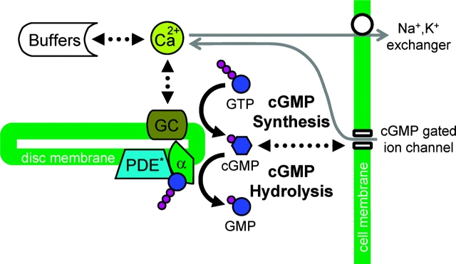
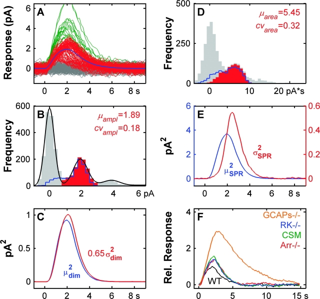
Single-photon responses (SPRs) in vertebrate rods are considerably less variable than expected if isomerized rhodopsin (R*) inactivated in a single, memoryless step, and no other variability-reducing mechanisms were available. We present a new stochastic model, the core of which is the successive ratcheting down of R* activity, and a concomitant increase in the probability of quenching of R* by arrestin (Arr), with each phosphorylation of R* (Gibson, S.K., J.H. Parkes, and P.A. Liebman. 2000. Biochemistry. 39:5738-5749.). We evaluated the model by means of Monte-Carlo simulations of dim-flash responses, and compared the response statistics derived from them with those obtained from empirical dim-flash data (Whitlock, G.G., and T.D. Lamb. 1999. Neuron. 23:337-351.). The model accounts for four quantitative measures of SPR reproducibility. It also reproduces qualitative features of rod responses obtained with altered nucleotide levels, and thus contradicts the conclusion that such responses imply that phosphorylation cannot dominate R* inactivation (Rieke, F., and D.A. Baylor. 1998a. Biophys. J. 75:1836-1857; Field, G.D., and F. Rieke. 2002. Neuron. 35:733-747.). Moreover, the model is able to reproduce the salient qualitative features of SPRs obtained from mouse rods that had been genetically modified with specific pathways of R* inactivation or Ca2+ feedback disabled. We present a theoretical analysis showing that the variability of the area under the SPR estimates the variability of integrated R* activity, and can provide a valid gauge of the number of R* inactivation steps. We show that there is a heretofore unappreciated tradeoff between variability of SPR amplitude and SPR duration that depends critically on the kinetics of inactivation of R* relative to the net kinetics of the downstream reactions in the cascade. Because of this dependence, neither the variability of SPR amplitude nor duration provides a reliable estimate of the underlying variability of integrated R* activity, and cannot be used to estimate the minimum number of R* inactivation steps. We conclude that multiple phosphorylation-dependent decrements in R* activity (with Arr-quench) can confer the observed reproducibility of rod SPRs; there is no compelling need to invoke a long series of non-phosphorylation dependent state changes in R* (as in Rieke, F., and D.A. Baylor. 1998a. Biophys. J. 75:1836-1857; Field, G.D., and F. Rieke. 2002. Neuron. 35:733-747.). Our analyses, plus data and modeling of others (Rieke, F., and D.A. Baylor. 1998a. Biophys. J. 75:1836-1857; Field, G.D., and F. Rieke. 2002. Neuron. 35:733-747.), also argue strongly against either feedback (including Ca2+-feedback) or depletion of any molecular species downstream to R* as the dominant cause of SPR reproducibility.

Figure 1.

(A) Stochastic model of “front-end” reaction (eEqs. 1–3e). Model showing the stochastic activation of G and PDE, the inactivation of R*, G*, and G·PDE*, as well as the competition between Arr, G, and RK for R_n*, where n (0 ≤ n ≤ 7) is the number of times R* has been phosphorylated at any given point in time. Three mutually exclusive pathways for R_n* are depicted: (1) R* inactivation by Arr-capping, the probability of which increases with n (Gibson et al., 2000); (2) phosphorylation of R* by RK, the probability of which is assumed to decrease with n; or (3) activation of G-protein, the probability of which decreases with n (Gibson et al., 2000). The gray arrows indicate the “return” pathways for R*, i.e., when it is released from G protein or RK. Phosphorylation-dependent reactions are indicated by purple arrows. (B) Activation and inactivation of PDE (Eq. 8a–c). Activated transducin (G_α·GTP) binds to the PDEγ subunit (Eq. 8a). Inhibition by the PDEγ subunit is then relieved (Eq. 8b), yielding activated transducin–PDE* complex. For simplicity, inactivation of PDE* is assumed to occur in a single step (Eq. 8c; see text for details).

Figure 2.

Schematic representation of differential equation model of “back-end”. Model showing reactions subsequent to PDE activation, including cGMP-hydrolysis and synthesis, channels closure, Ca²⁺ feedback, Ca²⁺-buffering. These reactions were simulated as deterministic reactions with differential equations.

Figure 3.

The empirical data sets with which model results are compared. The first five panels (A–E) show analyses of original data from Whitlock and Lamb (1999). (A) Waveforms of 101 SPRs (red) and 51 MPRs (green), as well as 161 waveforms judged to be failures (gray). We have reanalyzed Whitlock and Lamb's data using the methodology described in materials and methods. The solid blue curve is the ensemble mean of the SPRs. (B) Histogram of amplitudes for all recording epochs shown in A. Amplitude for each response was calculated as described in materials and methods. The solid black curve shows the result of fitting a sum-of-Gaussians model to the data, yielding estimates of the σ and μ of each of the presumed underlying distributions. These parameters were then used to classify responses as either failures, SPRs, or MPRs by determining upper and lower amplitude limits beyond which the probability that a response was an SPR fell below 50%. The CV for SPR amplitudes identified in this manner (red overlay in histogram) was 0.15. (C) Comparison between the light-evoked ensemble variance increase (red) and the square of the ensemble mean (blue). The variance increase was calculated by subtraction of the variance of the failures from the variance of all responses. Variance was scaled by a factor of 0.53 to match the mean squared. (D) Histogram of response areas for all responses (failures, SPRs and MPRs) as classified from the amplitude histogram in B. The area for each response was calculated by integrating the response over the 9 s after the each stimulus presentation. For the failures, ∼50% of the responses had negative areas, as expected. The CV for area of the SPRs (red overlay) was 0.36. (E) The time-dependent residual variance of SPRs (σ_SPR ²−σ_failure ²; red curve) and the square of the mean SPR (blue curve). The SPRs were categorized from the model fit to the amplitude histogram as in B. The SPR variance is approximately an order of magnitude smaller than the square of the mean response until after the peak of the mean response, peaks much later than the mean and is broader. F and G reproduce data from Fig. 14 of Rieke and Baylor (1998a), showing the effects of lowering transduction gain in the presence of normal, control levels of ATP (500 μM) or low ATP (20 μM) levels in truncated toad rod outer segments. Responses are averages of 10–15 trials, each eliciting ∼10 photoisomerizations. For each ATP condition, GTP concentration was decreased by a factor of 2.5 (control GTP: blue; low GTP: red). With normal ATP (F), lowering GTP caused the dim-flash response amplitude to decrease with no effect on the response kinetics. In low ATP (G), the same GTP manipulation decreased response amplitude and slowed the response. Rieke and Baylor (1998a) interpreted these results to imply that neither phosphorylation nor arrestin-binding controlled the majority of rhodopsin's cumulative activity. Insets in panels F and G show the responses before peak amplitudes were equated. The peak amplitudes were, control ATP: 19 pA (control GTP), 11 pA (low GTP); low ATP: 23 pA (control GTP), 14 pA (low GTP). (H) The results of one study in which feedback synthesis of cGMP was genetically disrupted, plus three studies in which R* inactivation mechanisms were disrupted by genetic knockout or transgenic manipulation of mouse rods. (Red) Arr−/− (Xu et al., 1997, Mn of 21 responses); (Blue) RK−/− (Chen et al., 1999, mean of 14 responses); (Green) transgenic disabling of six phosphorylation sites on rhodopsin (Mendez et al., 2000, CSM responses, mean of 10 responses; see text for details); (Orange) GCAPs−/− (Burns et al., 2002, mean of 31 rod responses). The WT responses from each of these studies are shown as thin curves. The WT responses were scaled to the same relative peak amplitude (1.0), but the relationship to the corresponding genetically manipulated responses in each case was not altered. The actual mean WT SPR peak amplitude in each study was on the order of 0.3 - 0.6 pA.

Figure 4.

Predictions of sequential phosphorylation model. The model generates SPRs with empirical reproducibility (B–E) and captures all the other data, including the salient features of the transgenic and KO mouse rod data (H). The model responses include the addition of simulated recording and photoreceptor noise and response failures (materials and methods). All the analyses of the model responses were carried out using the same methodology as was applied to Whitlock and Lamb's data in Fig. 3. The CV of SPR amplitudes identified statistically (red overlay in B) was 0.16, nearly identical to the value obtained from the Whitlock and Lamb (1999) data (0.15; Fig. 3 B). The CV for SPR amplitudes when SPRs were identified perfectly (solid blue curve in B) was 0.20, illustrating that our statistical method of response classification was working well (see text for details). The SPR variability (CV _area = 0.38) was close the empirical value (0.36) from the Whitlock and Lamb data (compare panel D with Fig. 3 D). The CV _area for SPRs identified perfectly (0.42, blue curve in D) was close to the value for SPRs identified with our statistical method (0.38, red overlay in D). The inset in D shows the distribution of the number of phosphorylations at Arr-capping, with the vertical red line marking the mean (6.1). As in the data, the variance of the SPRs peaked much later than the squared mean of the SPRs (1.6 times later; E). The sequential phosphorylation model also reproduces the transduction gain manipulation data from Fig. 14 of Rieke and Baylor (1998a) (F and G). F shows the results of a simulation under the control ATP condition. The decrease in GTP by a factor of 2.5 (blue: control GTP; red: low-GTP) decreases transduction gain (shown in inset) without significantly altering the kinetics of the response (shown by the larger normalized curves). However, when ATP is lowered by a factor of 25 (G) as in Rieke and Baylor (1998a), the same GTP manipulation decreased the gain (inset) and slowed the kinetics of the response (compare with F and G, Fig. 3). The peak amplitudes of the responses shown in the two insets in F and G were, control ATP: 4.7 pA (control GTP), 2.6 pA (low GTP); low ATP: 9.6 pA (control GTP), 5.5 pA (low GTP). The absolute amplitudes were lower than those reported in Rieke and Baylor (1998a) because we simulated single-photon responses, not responses to 10 R*. These results show that, contrary to Rieke and Baylor's (1998a) interpretation of their data, this pattern of responses under nucleotide manipulation is not incompatible with phosphorylation dominating R* inactivation.

Figure 5.

Numerical simulations showing that phosphorylation dominates R* inactivation. Mean R* activity (defined as G* activations s⁻¹) in response to a single photon absorptions was simulated by recording the stochastic G–activation events associated with each of 1,000 SPRs under three conditions: (1) WT (i.e., using our sequential phosphorylation model; blue curve). Here, both phosphorylation and Arr-capping contribute to R* inactivation. (2) CSM (green curve). Both phosphorylation and Arr-quench are disabled. In the absence of phosphorylation, R* activity goes to a fixed, steady-state level close to the theoretical initial maximal R* activity of ∼146 G*/s (derived from Eq. 15, for n = 0). (3) Arr−/− (red curve). Arr-quench is disabled, but phosphorylation is not. Thus, this curve depicts the mean reduction in R* activity due to phosphorylation per se. These three R* activity curves demonstrate qualitatively that phosphorylation dominates R* inactivation at all times, including at the mean time of Arr-quench (vertical dotted line at 2.7 s). This was quantified in the following manner: For each of 1,000 Monte-Carlo trials under the WT condition, the fractional decrease in R* activity, due to phosphorylation alone, at the time of Arr-quench was measured. The average of these 1,000 values was taken as a measure of the mean fractional decrease of R* activity due to phosphorylation alone. The decrease in R* activity at measured in this way was 66%, with Arr-quench accounting for the remaining 34% of R* activity reduction.

Figure 6.

CV _ampl and CV_dur (but not CV _area) tradeoff as a function of R* inactivation kinetics in relation to kinetics of downstream reactions. A. Predicted CVs as a function of τ_PDE. Monte-Carlo simulations were run using seven different values of τ_PDE, ranging from 0.75 s (R* recovery highly rate-limiting) to 12 s (PDE* recovery highly rate-limiting). For each τ_PDE, the front-end parameters were adjusted so that the mean simulated dim-flash response closely matched the mean dim-flash response in the Whitlock and Lamb (1999) data, and the mean number of phosphorylations at Arr-binding was about the same as in the sequential phosphorylation model (so that the expected CV _area would approximately equal the CV _area for the sequential phosphorylation model). For the purposes of this analysis, CVs for SPR amplitude, duration, and area were calculated in the absence of noise; amplitude for each SPR was defined as the peak amplitude; and SPR duration was defined as the SPR area divided by the peak SPR amplitude. Thus, the resulting CVs will not exactly match those derived from the more empirically based methods used in the main analyses of the sequential phosphorylation model (see materials and methods). The full biochemical model clearly manifests the tradeoff behavior predicted from the limiting-case scenarios (see text). Only CV _area (open circles) is independent of what rate-limits recovery (CV _area is constant over all τ_PDE values). (B) Number of R* inactivation steps inferred from CVs in A. The number of inferred steps from A were calculated as 1/CV ². The number of steps inferred from the CV _area measures (open circles) match the actual number of R* inactivation steps used (X, dashed line), whereas CV _ampl and CV _dur severely overestimate the number of R* inactivation steps over most of the range of τ_PDE values.

Figure 7.

Early saturation (local depletion of PDE) can produce low SPR variability, but fails to account for other key data. Early saturation was achieved by restricting the total pool of locally available PDE to ∼300. R* activity was simulated as an all-or-none pulse of activity until inactivation. Inactivation occurred by arrestin binding immediately upon the first phosphorylation, so that inactivation was effectively a single step process, ensuring that only the PDE saturation could reduce SPR variability. The resulting measured CV _area (0.32; D) and CV _ampl (0.18; B) were low, close to empirical levels. In addition, the variance of the ensemble dim-flash responses was close to the square of the ensemble mean (C), and the individual simulated responses (A) look similar to the real data (Fig. 3 A). However, an early saturation model fails completely to reproduce the correct Arr−/−, RK−/−, and CSM response features; these all recover fully with nearly WT kinetics (F), in striking contrast to the data (Fig. 3 H). The predicted SPR variance peaks too early, and is too narrow (compare panel E with Fig. 3 E). In addition, this model produces an inordinate number of small-amplitude, small-area SPRs (solid blue curves in B and D showing the veridical distributions) that overlap substantially the distribution of response failures (gray distributions centered at zero on the abscissas in B and D). The variability of the veridical distributions is much higher (CV _ampl = 0.45 vs. 0.18; CV _area = 0.57 vs. 0.32, panels B and D) than the CVs derived when the responses are analyzed as empirical data.

Figure 8.

Consequences of single-step R* inactivation. R* activity was simulated as an all-or-none pulse of activity until inactivation. Inactivation occurred by arrestin binding immediately upon the phosphorylation, so that inactivation was effectively a single-step process. In all other respects, the model and analyses (including the addition of simulated noise) were the same as for the sequential phosphorylation model. Despite being able to reproduce a reasonable mean SPR (solid blue curve in A; compare with Fig. 3 A), this model fails to capture the critical features of the empirical data shown in Fig. 3. As expected, the responses exhibit a high degree of variability that is evident by inspection of the waveforms in panel A. This variability manifests as a severe mismatch between the σ_dim ² and μ_dim ² (C), and an inordinately high SPR variance (E). Because there is an unavoidable tradeoff between amplitude and duration variability that depends on the relative kinetics of the “front-end” and “back-end” phototransduction reactions, we cannot know in advance how much of the variability of R* lifetime will manifest in the SPR amplitudes. When the response amplitudes are analyzed as they were for the Whitlock and Lamb (1999) data and for the sequential phosphorylation model, the amplitude histogram shows clear multimodality, with a calculated SPR CV _ampl of 0.24. The amplitudes of responses identified statistically as SPRs are shown as a red overlay in B. Calculation of CV _area for SPRs identified from this amplitude histogram yields a relatively high value (0.77; red overlay, D), but substantially lower than the theoretically expected value of ∼1. However, as described in , the relatively low CV _ampl and CV _area are a consequence of the method of amplitude measurement and of classification of responses whenever the underlying response distributions are highly non-Gaussian. This is demonstrated in B and D where the response amplitudes and areas based on perfect identification of SPRs are shown by solid blue curves. The CV _ampl from this distribution is substantially larger (0.48), and the CV _area is now nearly one (0.97), as expected based on theory. Because the model inactivates immediately upon Arr-binding, the simulated Arr−/− response (F) is the same as the RK−/− (blue) and CSM (green), contrary to what is seen in the empirical Arr−/− data (Xu et al., 1997).

References

1. Arshavsky, V.Y., T.D. Lamb, and E.N. Pugh. 2002. G proteins and phototransduction. Annu. Rev. Physiol. 64:153–187. - PubMed
1. Aton, B.R., B.J. Litman, and M.L. Jackson. 1984. Isolation and identification of the phosphorylated species of rhodopsin. Biochemistry. 23:1737–1741. - PubMed
1. Baylor, D.A., T.D. Lamb, and K.W. Yau. 1979. Responses of retinal rods to single photons. J. Physiol. 288:613–634. - PMC - PubMed
1. Baylor, D.A., B.J. Nunn, and J.L. Schnapf. 1984. The photocurrent, noise and spectral sensitivity of rods of the monkey Macaca fascicularis. J. Physiol. 357:575–607. - PMC - PubMed
1. Burns, M.E., A. Mendez, J. Chen, and D.A. Baylor. 2002. Dynamics of cyclic GMP synthesis in retinal rods. Neuron. 36:81–91. - PubMed
Publication types