Biodiversity as spatial insurance in heterogeneous landscapes

Abstract

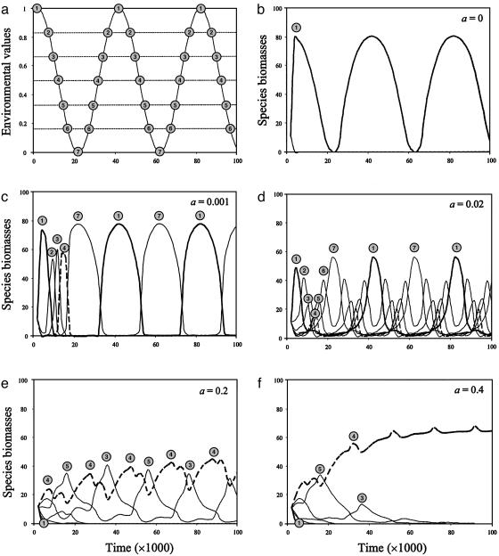
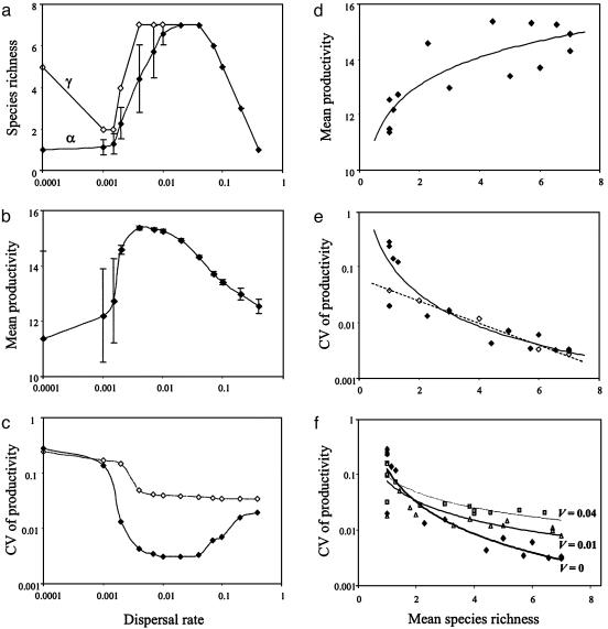
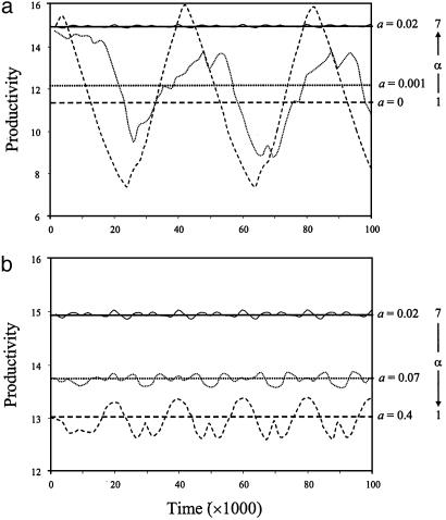
The potential consequences of biodiversity loss for ecosystem functioning and services at local scales have received considerable attention during the last decade, but little is known about how biodiversity affects ecosystem processes and stability at larger spatial scales. We propose that biodiversity provides spatial insurance for ecosystem functioning by virtue of spatial exchanges among local systems in heterogeneous landscapes. We explore this hypothesis by using a simple theoretical metacommunity model with explicit local consumer-resource dynamics and dispersal among systems. Our model shows that variation in dispersal rate affects the temporal mean and variability of ecosystem productivity strongly and nonmonotonically through two mechanisms: spatial averaging by the intermediate-type species that tends to dominate the landscape at high dispersal rates, and functional compensations between species that are made possible by the maintenance of species diversity. The spatial insurance effects of species diversity are highest at the intermediate dispersal rates that maximize local diversity. These results have profound implications for conservation and management. Knowledge of spatial processes across ecosystems is critical to predict the effects of landscape changes on both biodiversity and ecosystem functioning and services.

Fig. 1.

Environmental fluctuations (a) and dynamics of species biomasses for various dispersal rates (b–f) in community 1. In a, the time when each species is potentially the best competitor is indicated by its number in a gray circle, and the dashed horizontal lines show constant species trait values. In b–f, the numbers in gray circles indicate species identity, the bold solid line corresponds to the species that has the initial competitive advantage (species 1), and the dashed line corresponds to the species that has an average trait value (species 4).

Fig. 3.

Regional (γ) and mean local (α) species richness (a), temporal mean of ecosystem productivity (b), and coefficient of variation (CV) of ecosystem productivity through time (c) as functions of dispersal rate (mean ± SD across communities), and the resulting relationships between the temporal mean of ecosystem productivity (d) or the CV of ecosystem productivity (e and f) and mean local species richness. In d, the curve fitted to the data is a logarithmic function (r² = 0.71). In c and e, filled diamonds correspond to the original model in which both dispersal rate and species diversity are allowed to vary. In c, open diamonds show the results for the case in which the dispersal rate varies while local species richness is held constant at a single species (species 1). In e, open diamonds show the results for the case in which local species richness varies while the dispersal rate is held constant at an intermediate value (a = 0.02). In this scenario, species richness was varied by removing species sequentially from species 7 to species 2. The curves fitted to the data are a power function for filled diamonds (solid line, r² = 0.84) and an exponential function for open diamonds (dotted line, r² = 0.98). In f, a normally distributed random deviate with zero mean and variance (V) has been superimposed onto the periodic environmental fluctuations E_j(t) at each time step. Filled diamonds, V = 0 (no noise); open triangles, V = 0.01; gray squares, V = 0.04.

Fig. 2.

Temporal fluctuations and temporal mean of ecosystem productivity for various dispersal rates and corresponding levels of local species diversity, α. In a, the dispersal rate a increases from zero to intermediate values (a = 0, dashed line; a = 0.001, dotted line; a = 0.02, solid line). In b, it further increases from intermediate to high values (a = 0.02, solid line; a = 0.07, dotted line; a = 0.4, dashed line). Time averages (calculated when species biomasses settled into a regular pattern in time) are indicated by horizontal lines. Note that a and b have different scales on the y axis, for clarity.

References

1. Loreau, M., Naeem, S., Inchausti, P., Bengtsson, J., Grime, J. P., Hector, A., Hooper, D. U., Huston, M. A., Raffaelli, D., Schmid, B., et al. (2001) Science 294 804–808. - PubMed
1. Kinzig, A. P., Pacala, S. W. & Tilman, D., eds. (2002) The Functional Consequences of Biodiversity: Empirical Progress and Theoretical Extensions (Princeton Univ. Press, Princeton).
1. Loreau, M., Naeem, S. & Inchausti, P., eds. (2002) Biodiversity and Ecosystem Functioning: Synthesis and Perspectives (Oxford Univ. Press, Oxford).
1. Tilman, D., Knops, J., Wedin, D., Reich, P., Ritchie, M. & Siemann, E. (1997) Science 277 1300–1302.
1. Hector, A., Schmid, B., Beierkuhnlein, C., Caldeira, M. C., Diemer, M., Dimitrakopoulos, P. G., Finn, J. A., Freitas, H., Giller, P. S., Good, J., et al. (1999) Science 286 1123–1127. - PubMed
Publication types