Effects of skull thickness, anisotropy, and inhomogeneity on forward EEG/ERP computations using a spherical three-dimensional resistor mesh model

Abstract

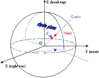
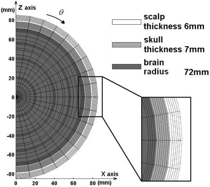
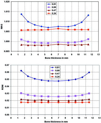
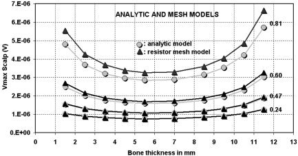
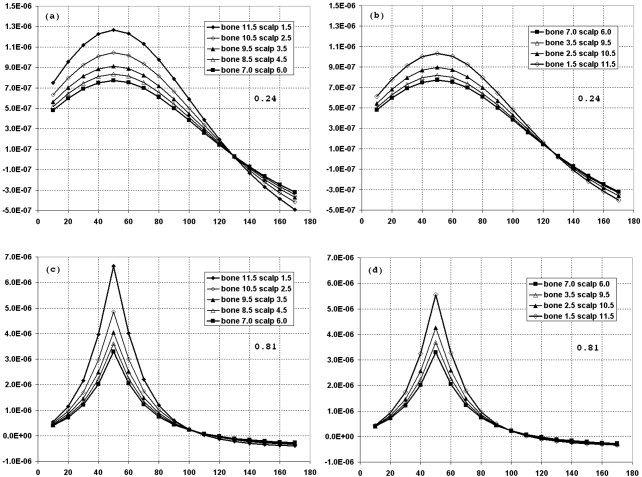
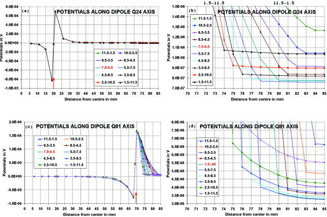
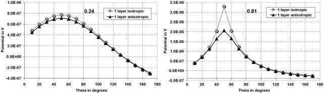
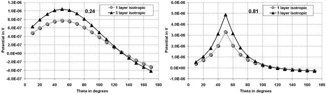
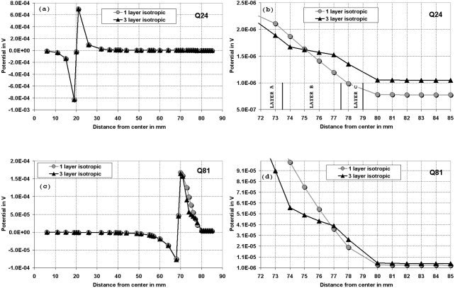
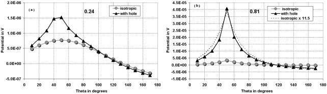
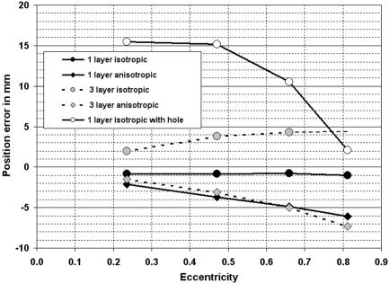
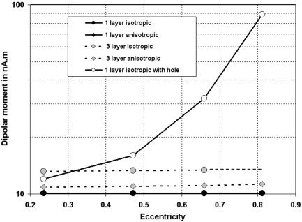
Bone thickness, anisotropy, and inhomogeneity have been reported to induce important variations in electroencephalogram (EEG) scalp potentials. To study this effect, we used an original three-dimensional (3-D) resistor mesh model described in spherical coordinates, consisting of 67,464 elements and 22,105 nodes arranged in 36 different concentric layers. After validation of the model by comparison with the analytic solution, potential variations induced by geometric and electrical skull modifications were investigated at the surface in the dipole plane and along the dipole axis, for several eccentricities and bone thicknesses. The resistor mesh permits one to obtain various configurations, as local modifications are introduced very easily. This has allowed several head models to be designed to study the effects of skull properties (thickness, anisotropy, and heterogeneity) on scalp surface potentials. Results show a decrease of potentials in bone, depending on bone thickness, and a very small decrease through the scalp layer. Nevertheless, similar scalp potentials can be obtained using either a thick scalp layer and a thin skull layer, and vice versa. It is thus important to take into account skull and scalp thicknesses, because the drop of potential in bone depends on both. The use of three different layers for skull instead of one leads to small differences in potential values and patterns. In contrast, the introduction of a hole in the skull highly increases the maximum potential value (by a factor of 11.5 in our case), because of the absence of potential drop in the corresponding volume. The inverse solution without any a priori knowledge indicates that the model with the hole gives the largest errors in both position and dipolar moment. Our results indicate that the resistor mesh model can be used as a robust and user-friendly simulation tool in EEG or event-related potentials. It makes it possible to build up real head models directly from anatomic magnetic resonance imaging without tessellation, and is able to take into account head heterogeneities very simply by changing volume elements conductivity. Hum. Brain Mapping 21:84-95, 2004.

Figure 1

Q‐axis and dipole plane used for the simulations. In Cartesian coordinates, x‐axis is pointing to the right ear, y‐axis to nose and z‐axis to the top of the head. In spherical coordinates, angle θ is defined versus z‐axis and ϕ is the angle toward x‐axis of the projection in the horizontal XOY plane. We call Q‐axis the line through the centre of the sphere oriented to θ = ϕ = 50 degrees. Q81, for instance, means that the dipole origin is at 69 mm from the centre for a standard head radius of 85 mm, corresponding to an eccentricity of 0.81.

Figure 2

Cross section of half of the spherical resistor mesh, at ϕ = 0 degrees (sagittal right view). Each segment represents a resistor. The nodes of the mesh correspond to the intersections of the segments. Skull and scalp are sampled with very thin layers to study their internal potential distribution.

Figure 3

Application of the dipole in the resistor mesh model. The quasi‐punctual dipole of the analytic model, placed at node N, is modeled by two current sources (−i and +i) plugged between nodes (N−1) and (N+1) in the resistor mesh model. These nodes are distant from L mm so that the dipolar moment is M = iL.

Figure 4

MAG and RDM for scalp potentials in the resistor mesh model versus the three‐sphere head analytic model for four eccentricities (0.24, 0.47, 0.66, and 0.81) and 10 skull thicknesses from 1.5–11.5 mm.

Figure 5

Maximum scalp potential values obtained with the resistor mesh model and with the three‐sphere head analytic model, for four eccentricities (0.24, 0.47, 0.66, and 0.81) and 10 skull thicknesses from 1.5–11.5 mm. Dipolar moment is kept constant (10 nA.m).

Figure 6

Surface potentials in the dipole plane for two eccentricities and 10 skull thickness. A: Eccentricity 0.24, bone thickness 11.5–7.0 mm. B: Eccentricity 0.24, bone thickness 7.0–1.5 mm. C: Eccentricity 0.81, bone thickness 11.5–7.0 mm. d: Eccentricity 0.81, bone thickness 7.0 to 1.5 mm. Abscissa θ varies from 10–170 degrees.

Figure 7

Potentials inside the 3D resistor mesh model. A: Along Q‐axis at 0.24 eccentricity (Q24). B: Along Q24 axis (zoomed) in skull and scalp layers. C: Along Q‐axis at 0.81 eccentricity (Q81). D: Along Q81 axis (zoomed) in skull and scalp layers.

Figure 8

Surface potentials in the dipole plane for the three‐sphere model using one‐layer isotropic skull and one‐layer anisotropic skull.

Figure 9

Surface potentials in the dipole plane for one‐layer isotropic skull and for three‐layer isotropic skull.

Figure 10

Potentials along Q‐axis dipole. A: Q24 for one‐ and three‐layer isotropic skull. B: Q24 zoomed in skull and scalp. C: Q81 for 1 and three‐layer isotropic skull. D: Q81 zoomed in skull and scalp.

Figure 11

Surface potentials in the dipole plane with or without a hole in the skull. The three‐sphere isotropic head model is modified locally for eccentricity 0.24 (a) and eccentricity 0.81 (b). The dot curve in (b) corresponds to the potentials of the isotropic curve magnified by a factor of 11.5.

Figure 12

Position error of inverse solution using Besa. Input data are simulated surface potentials taken at nodes corresponding to a 61‐electrode cap (10/20 system). With the three‐layer isotropic model, the result at eccentricity 0.81 has not been plotted because the dipole would have been localized in bone, which is impossible.

Figure 13

Dipole moment of inverse solution using Besa. Input data are the simulated surface potentials taken at nodes corresponding to a 61‐electrode cap (10/20 system). The correct dipolar moment to find is 10 nA.m (one‐layer anisotropic is hidden by one‐layer isotropic).

References

1. Akhtari M, Bryant HC, Mamelak AN, Flynn ER, Heller L, Shih JJ, Mandelkern M, Matlachov A, Ranken DM, Best ED, DiMauro MA, Lee RR, Sutherling WW (2002): Conductivities of three‐layer live human skull. Brain Topogr 14: 151–167. - PubMed
1. Ary JP, Klein SA, Fender DH (1981): Location of sources of evoked scalp potentials: corrections for skull and scalp thicknesses. IEEE Trans Biomed Eng 28: 447–452. - PubMed
1. Awada KA, Jackson DR, Williams JT, Wilton DR, Baumann SB, Papanicolaou AC (1997): Computational aspects of finite element modeling in EEG source localization. IEEE Trans Biomed Eng 44: 736–752. - PubMed
1. Benar CG, Gotman J (2002): Modeling of post‐surgical brain and skull defects in the EEG inverse problem with the boundary element method. Clin Neurophysiol 113: 48–56. - PubMed
1. Bertrand O, Thevenet M, Perrin F, Pernier J (1992): Effects of skull holes on the scalp potential distribution evaluated with a finite element method. Proceedings of the 14th International Conference of the IEEE Engineering in Medicine and Biology Society, Lyon. p 42–45.
LinkOut - more resources