The genetics of geometry

Abstract

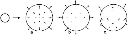
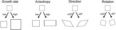
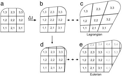
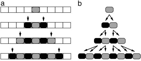
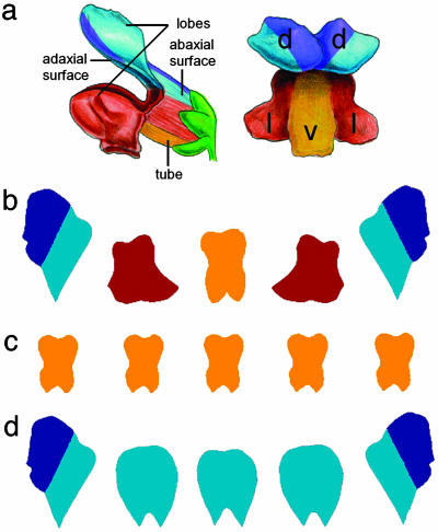
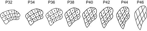
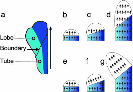
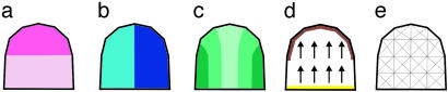
Although much progress has been made in understanding how gene expression patterns are established during development, much less is known about how these patterns are related to the growth of biological shapes. Here we describe conceptual and experimental approaches to bridging this gap, with particular reference to plant development where lack of cell movement simplifies matters. Growth and shape change in plants can be fully described with four types of regional parameter: growth rate, anisotropy, direction, and rotation. A key requirement is to understand how these parameters both influence and respond to the action of genes. This can be addressed by using mechanistic models that capture interactions among three components: regional identities, regionalizing morphogens, and polarizing morphogens. By incorporating these interactions within a growing framework, it is possible to generate shape changes and associated gene expression patterns according to particular hypotheses. The results can be compared with experimental observations of growth of normal and mutant forms, allowing further hypotheses and experiments to be formulated. We illustrate these principles with a study of snapdragon petal growth.

Fig. 1.

Velocity fields for a growing disk. (a) Isogonic growth with velocities shown relative to the center. (b) Growth mainly near the rim with velocities shown relative to the center. (c) Isogonic growth with velocities shown relative to the base of the disk.

Fig. 2.

Four types of regional parameter for describing growth properties.

Fig. 3.

Initial shape with nine regions (a) grows during a time interval Δt to a new shape (b). With a Lagrangian specification, the same material points are progressively followed, leading to a deformed grid (c). With an Eulerian specification, regions are redefined at each time step according to a fixed coordinate system (d), leading to further regions being added to a regular grid (e).

Fig. 4.

Growth in module number, illustrated with a 1D filament. (a) For cellular automata, the array is predefined, and modules are added by accretion (arrows). (b) In L-systems, the array grows in parallel with subdivision of modules.

Fig. 5.

(a) Core gene regulation network that controls heterocyst differentiation in an Anabaena filament. Nondiffusing protein HetR is responsible for the maintenance of the heterocyst state. Diffusing protein PatS inhibits differentiation of new heterocysts in the neighborhood of the existing ones. Red indicates high concentration of HetR, and dark blue indicates high concentration of PatS (courtesy of Carla Davidson, University of Calgary). (b–d) Development of an Anabaena filament, simulated by using an L-system model based on ref. . Vertical bars above filaments indicate concentrations of HetR protein; bars below filaments indicate concentrations of PatS protein. High concentration of HetR (red) indicates heterocysts. (b) Two heterocysts separated by a sequence of vegetative cells. (c) Vegetative cells grow and divide, moving the heterocysts apart. As a result, the concentration of inhibitor near the center of the filament decreases and the concentration of the activator increases, leading to differentiation of a new heterocyst. (d) The new heterocyst modifies the distribution of the inhibitor, which prevents clustering of heterocysts.

Fig. 6.

Model for coupling cell polarity to direction of morphogen flow. Morphogen molecules M diffuse (or are transported) in and out of the cell, whereas tally molecules (black dots) are localized at the cell membrane. The gradient of M is such that there is a net flow from the bottom of the cell to the top (vertical black arrows). M also crosses the membrane in the opposite way, but to a slightly lesser extent (gray arrows). Passage of M across the cell membrane is coupled to the movement (or synthesis/degradation or release/capture) of a tally molecule so that the tally molecule is transported across the membrane in the opposite direction to M. (a) Initially there is an equal concentration of tally molecules on each side of the membrane. (b) With time, the internal concentration of tally molecules increases at the top and decreases at the bottom of the cell until equilibrium is reached. The distribution of tally molecules would change gradually when the gradient of M changes orientation, leading to a change in cell polarity.

Fig. 7.

(a) Rectangle with isotropic growth rate increasing exponentially from left to right gives a curved final shape. (b) Flat disk with isotropic growth rate greater at the margins than at the center results in bending out of the plane and a wavy edge.

Fig. 8.

Modeling growth with springs. Growth of each region shown in a is implemented by changing the resting lengths of the springs and letting them equilibrate (b), which is equivalent to inserting extra lengths of material (gray segments in b) into the springs.

Fig. 9.

(a) Antirrhinum flower shown in side view (Left) or face view (Right). Regions are color coded as blue (dorsal), brown (lateral), and yellow (ventral). The dorsal half of the dorsal petal is shown in darker blue [reproduced with permission from ref. (Copyright 2003, Nature Publishing Group, www.nature.com).] (b–d) Flattened petal lobes of wild-type (b), cyc dich double mutant (c), and mutant expressing CYC ectopically (d).

Fig. 10.

Shape changes in petal lobe from early to late stages. Lines show main directions of growth for each region at each stage when anisotropy was >1.05 per cell division. Petals have been scaled to the same size and aligned such that the average direction of growth is vertical. The scaling factor in area between P32 and P46 is 105.

Fig. 11.

(a) Flattened dorsal petal color coded as in Fig. 9 showing boundary between tube and lobe. Vertical arrow indicates the proximodistal axis. (b–d) Change in shape when growth direction is continuously coordinated along the whole petal (arrows arbitrarily shown pointing up rather than down). Lobe is white and tube is blue, with dorsal regions darker blue. Initially, the lobe is bilaterally symmetrical (b). Dorsal side of the tube grows preferentially, resulting in a change in the orientation of the tube-lobe boundary (c). As growth direction is maintained parallel to the proximodistal axis, anisotropic growth results in the lobe becoming asymmetric (d). (e and f) Change in shape if the direction of growth becomes fixed at an early stage. Initially (e), growth direction is vertical as in b, but, as the tube-lobe boundary changes orientation, the direction of growth within the lobe rotates together with the lobe (f), leading to a bilaterally symmetrical lobe (g).

Fig. 12.

Wild-type dorsal petal at an early stage of development with regional identities distinguished along different axes. (a) The petal is divided along the proximodistal axis into a tube (pale-pink) and lobe (dark-pink) region. (b) The petal is divided along the dorsoventral axis of the flower into a more dorsal (dark-blue) and lateral (light-blue) half. (c) The petal is divided along its mediolateral axis into middle (light-green), intermediate (mediumgreen), and side (dark-green) regions. (d) A region is defined at the base of the petal (bright yellow) that provides a source of polarizing morphogen that diffuses (arrows) toward a distal sink (brown). (e) Subdivision of petal into finite elements.

Fig. 13.

Final petal shapes resulting from growth models operating on the starting shape shown in Fig. 12. Only distinctions along the dorsoventral axis are color-coded. Tube-lobe boundary is highlighted in black, and the main directions of growth is indicated with short pale-yellow lines. (a) Model of wild-type dorsal petal with direction determined by a polarizing morphogen acting continuously during growth. (b) Same as a except that dark blue has been removed, capturing the development of the backpetal mutant.

References

1. Lawrence, P. A. (1992) The Making of a Fly (Blackwell Scientific, Oxford).
1. Wolpert, L., Brockes, J., Jessell, T., Lawrence, P. & Meyerowitz, E. (1998) Principles of Development (Oxford Univ. Press, Oxford).
1. Coen, E. (2000) The Art of Genes (Oxford Univ. Press, Oxford).
1. Teleman, A., Strigini, M. & Cohen, S. M. (2001) Cell 105, 559–562. - PubMed
1. Steeves, T. A. & Sussex, I. M. (1989) Patterns in Plant Development (Cambridge Univ. Press, Cambridge, U.K.).
Publication types
LinkOut - more resources