Why is spatial stereoresolution so low?

Abstract

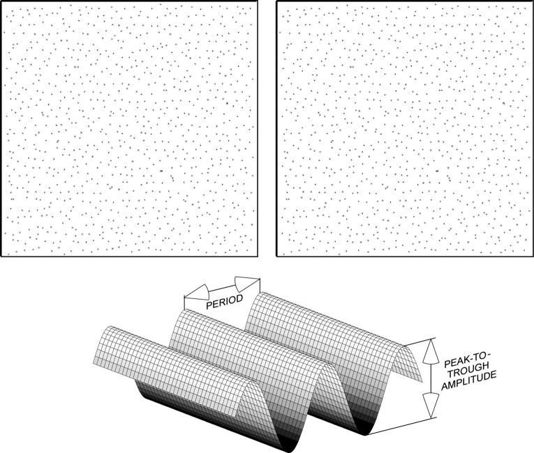
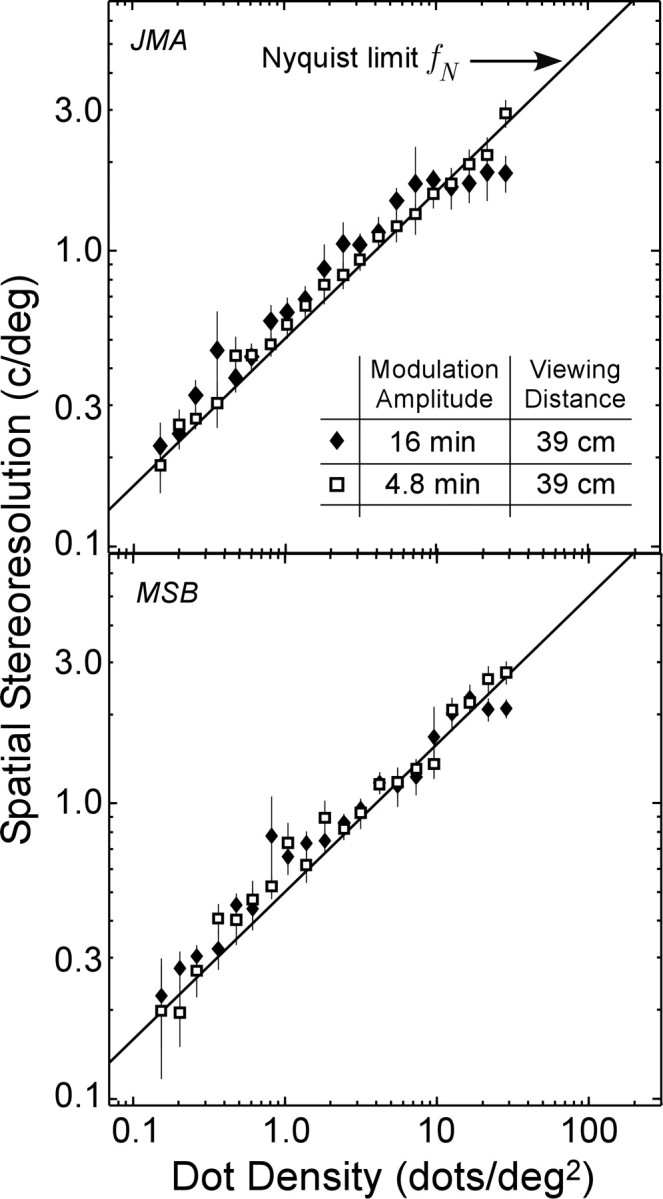
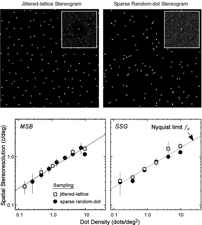
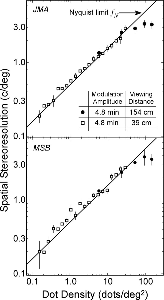
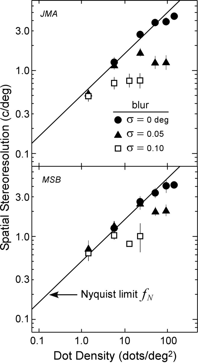
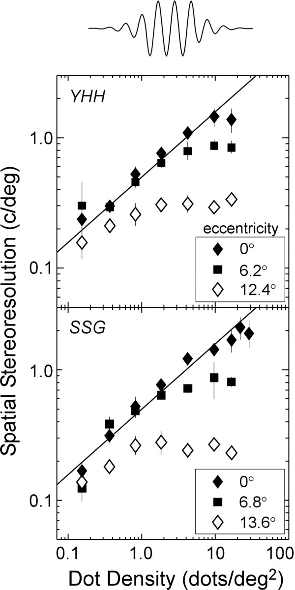
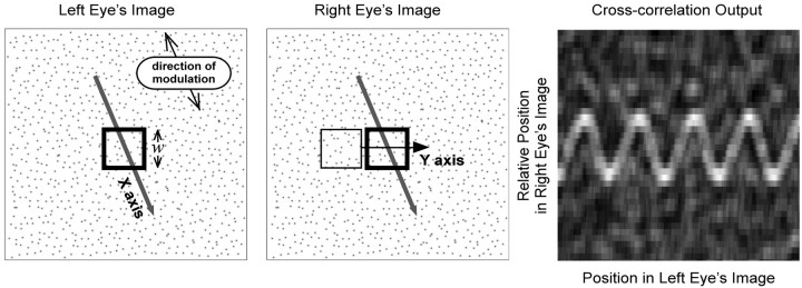
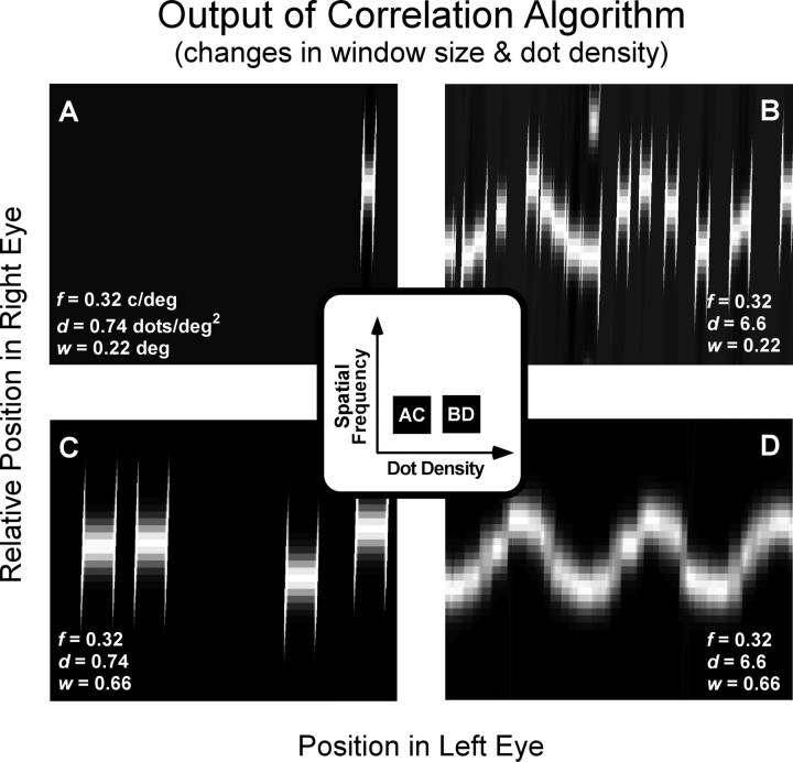
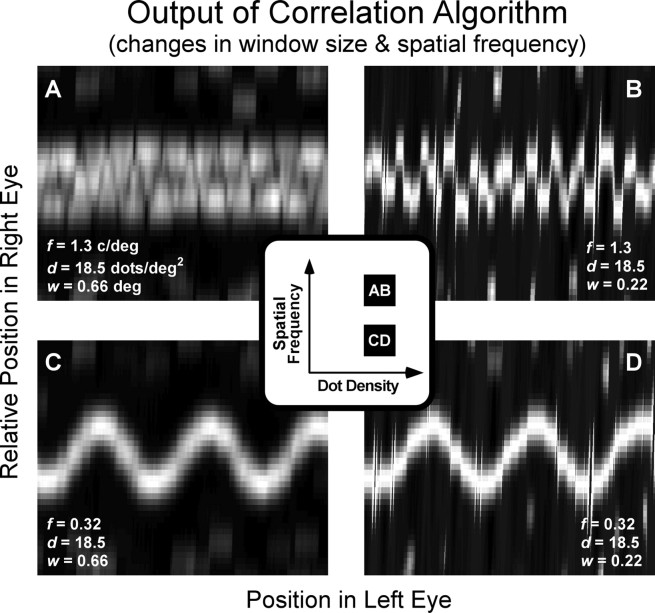
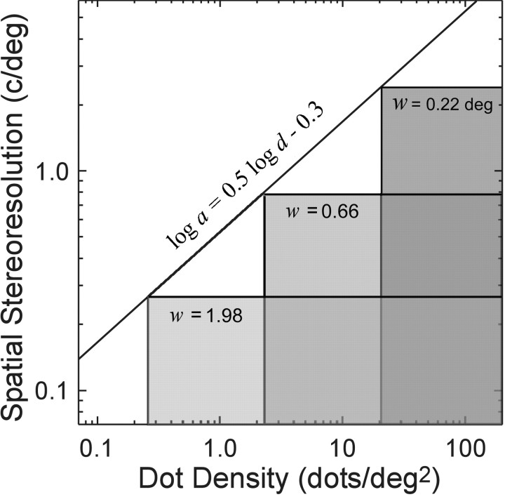
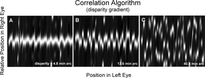
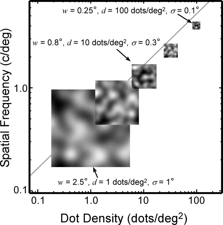
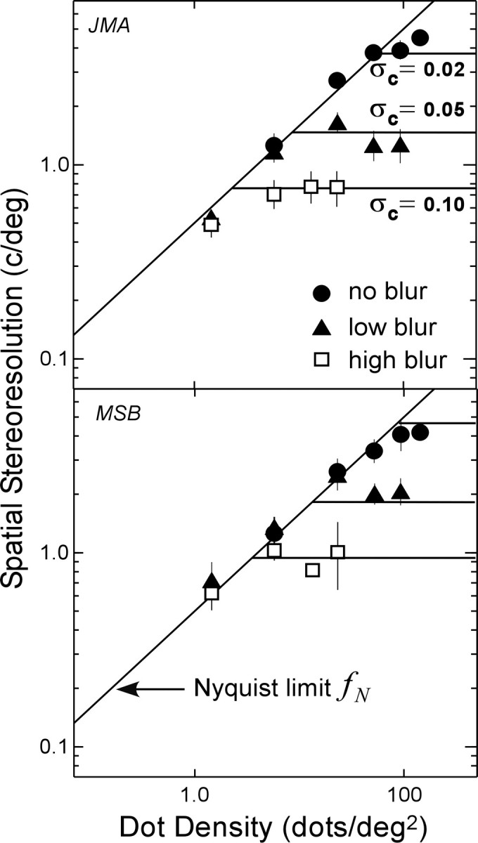
Spatial stereoresolution (the finest detectable modulation of binocular disparity) is much poorer than luminance resolution (finest detectable luminance variation). In a series of psychophysical experiments, we examined four factors that could cause low stereoresolution: (1) the sampling properties of the stimulus, (2) the disparity gradient limit, (3) low-pass spatial filtering by mechanisms early in the visual process, and (4) the method by which binocular matches are computed. Our experimental results reveal the contributions of the first three factors. A theoretical analysis of binocular matching by interocular correlation reveals the contribution of the fourth: the highest attainable stereoresolution may be limited by (1) the smallest useful correlation window in the visual system, and (2) a matching process that estimates the disparity of image patches and assumes that disparity is constant across the patch. Both properties are observed in disparity-selective neurons in area V1 of the primate (Nienborg et al., 2004).

Figure 1.

Example and schematic of the experimental stimulus. The top row is a stereogram like the ones used in the experiments reported here. If you cross-fuse, you will see a sinusoidal depth corrugation that is rotated 20° counterclockwise from horizontal. The bottom panel is a schematic of the disparity waveform stimulus.

Figure 2.

Spatial stereoresolution as a function of dot density. The highest discriminable corrugation frequency is plotted as a function of the dot density of the stereogram. Each panel shows results from one observer (JMA in the top panel and MSB in the bottom panel). Results from two more observers are shown in Figure S1 in the supplementary on-line material. The filled diamonds represent the measured resolution when the disparity amplitude was 16 min arc, and the open squares represent the resolution when the amplitude was 4.8 min arc. The solid lines represent the Nyquist sampling limit f_N of the dot pattern (Eq. 1). Viewing distance was 39 cm. The error bars are ±1 SD.

Figure 3.

Jittered-lattice and sparse random-dot stereograms. Top row, Half images associated with the two types of stereograms. Bottom row, Spatial stereoresolution as a function of dot density for the two types of stereograms. Top left, The larger image is a monocular image from a jittered-lattice stereogram such as the ones used in the current study. See Materials and Methods for details. The inset is the amplitude spectrum of this monocular image. Top right, The larger image is a monocular image from a sparse random-dot stereogram such as the ones used by Nienborg et al. (2004). The inset is the amplitude spectrum of this monocular image. The two bottom panels plot the highest discriminable corrugation frequency as a function of dot density. Each panel shows results from one observer (MSB and SSG). The open squares represent resolution for a jittered-lattice stereogram (Fig. 1 and top left panel), and filled circles represent resolution for a sparse random-dot stereogram (top right panel). Disparity amplitude was 4.8 min arc, viewing distance was 39 cm, and stimulus duration was 600 msec. The solid lines represent the Nyquist sampling limit f_N of the dot pattern (Eq. 1). The error bars are ±1 SD.

Figure 4.

Spatial stereoresolution as a function of dot density at two viewing distances (two observers, JMA and MSB). The open squares represent the measured resolution at a viewing distance of 39 cm, and the filled circles represent the resolution at a distance of 154 cm. The solid lines again represent the Nyquist sampling limit (Eq. 1). Disparity amplitude was 4.8 min arc. Results from two more observers are shown in Figure S2 in the supplementary on-line material. The error bars are ±1 SD.

Figure 5.

Spatial stereoresolution as a function of dot density with different amounts of stimulus blur (two observers, JMA and MSB). The filled circles represent the measured resolution with no blur, the filled triangles represent the resolution at the low-blur level, and open squares represent the resolution at the high-blur level at the viewing distance of 154 cm. The solid lines again represent the Nyquist limit. Disparity amplitude was 4.8 min arc. The error bars are ±1 SD.

Figure 6.

Spatial stereoresolution as a function of dot density at different retinal eccentricities (two observers, YHH and SSG). The stimuli were a full field of random dots with a small region in which the disparity modulation was present. A cross-section of the disparity modulation is shown at the top. The filled diamonds represent the measured resolution at fixation (eccentricity, 0°), the filled squares represent the resolution at the intermediate eccentricity, and the open diamonds represent the resolution at the large eccentricity. The solid lines again represent the Nyquist limit. Disparity amplitude was 16 min arc, viewing distance was 39 cm, and stimulus duration was 250 msec. Results from one more observer are shown in Figure S3 in the supplementary on-line material. The error bars are ±1 SD.

Figure 7.

Schematic of the correlation algorithm for binocular matching. The left and middle panels are the images presented to the left and right eye. The corrugation waveform is oriented 20° counterclockwise from horizontal. A square correlation window was placed in the image of the left eye (thick square); its width and height were w. That window was moved on a line (oblique arrow) through the middle of the image and in a direction orthogonal to disparity corrugation. For each position of the left eye window, a square window was placed in the right eye image (thin square); its width and height were also w. We restricted the movement of the window of the right eye to a horizontal line (horizontal arrow) through the midpoint of the window of the left eye. For each position of the window of the left eye, we computed the cross-correlation between the two windowed images (Eq. 3). The right panel shows the output of the algorithm. The abscissa is the position of the window in the left eye image (along the oblique arrow), and the ordinate is the relative position of the window in the right eye image (along the horizontal arrow) (i.e., horizontal disparity). For ease of viewing, the scale of the ordinate has been magnified relative to the scale of the abscissa. Correlation is represented by intensity, brighter values corresponding to higher correlations. In this particular case, the algorithm produced a sinusoidal ridge of high correlation corresponding to the sinusoidal disparity signal.

Figure 8.

Effect of window size and dot density on binocular matching by interocular correlation. Each panel displays the correlation as a function of position of the window in the left and right eyes. The scale of the ordinate has been magnified relative to the scale of the abscissa. The inset represents the spatial frequencies and dot densities for the stimuli that were used to generate the outputs shown in the four panels. A and C show outputs for the same stimulus: corrugation frequency, 0.32 cycle/°; dot density, 0.74 dots/deg². B and D show outputs for a stimulus with a higher dot density of 6.6 dots/deg². A and B have a correlation window of 0.22 × 0.22°, and C and D have a window of 0.66 × 0.66°.

Figure 9.

Effect of window size and corrugation frequency on binocular matching by interocular correlation. The scale of the ordinate has been magnified relative to the scale of the abscissa. The inset represents the spatial frequencies and dot densities for the stimuli that were used to generate the outputs shown in the four panels. A and B show outputs for the same stimulus: corrugation frequency, 1.3 cycles/°; dot density = 18.5 dots/deg². C and D show outputs for a stimulus with a lower corrugation frequency of 0.32 cycle/°. A and C have a correlation window of 0.66 × 0.66°, and B and D have a window of 0.22 × 0.22°.

Figure 10.

Critical spatial frequencies and dot densities for different window sizes. The correlation algorithm exhibits an asymptotic resolution a, which is inversely proportional to window width w. The top edges of the tall, intermediate, and short shaded areas represent that asymptotic frequency for correlation window sizes of 0.22 × 0.22°, 0.66 × 0.66°, and 1.98 × 1.98°, respectively. The correlation algorithm also exhibits a limiting dot density d that is inversely proportional to window area. The left edges of the tall, intermediate, and short shaded areas represent that critical density for correlation windows of 0.22 × 0.22°, 0.66 × 0.66°, and 1.98 × 1.98°, respectively. The diagonal line is a plot of Equation 6, which has a slope of 0.5 in this log-log plot. The shaded areas represent the combinations of corrugation frequency and dot density for which each of the three correlation windows would estimate disparity accurately.

Figure 11.

Effect of disparity gradient on binocular matching by interocular correlation. The corrugation frequency and dot density of the stimuli are the same for each panel (f = 1.3 cycles/°; d = 18.5 dots/deg²), and the size of the correlation window is the same (w = 0.22°). The disparity amplitude increases nearly ninefold from the left panel to the right: amplitude, 4.8 min arc (A), 13.6 min arc (B), and 40.8 min arc (C).

Figure 12.

Effect of low-pass spatial filtering and scale invariance of spatial stereoresolution. The five insets represent a monocular image as seen by a correlation window. Dot density in the inset images ranges from 1 to 100 dots/deg² from left to right. The width of the correlation window is inversely proportional to dot density: , large enough to include on average approximately six samples per window. The low-pass spatial filter is represented by an isotropic Gaussian. The SD σ of the Gaussian is proportional to w: σ = w/2.5. The intensity variation expressed in cycles per window is constant across the insets (apart from random variation in the stimulus) because of the proportionalities between the dot density d, window size w, and blur constant σ. The diagonal line represents the Nyquist limit. Our data suggest that stereoresolution expressed in cycles per degree would fall along a positive diagonal for these stimuli, so we placed the insets on a diagonal of the same slope as the Nyquist limit, but below the limit.

Figure 13.

Observed and predicted stereoresolution as a function of blur. The data points are the same as the ones in Figure 5 (two observers, JMA and MSB). Filled circles represent resolution when no external blur was added to the stimulus. Filled triangles represent resolution when we added external blur with a space constant of 0.05° by placing a diffusion screen in front of the display. Open squares represent resolution when we added external blur with a space constant of 0.10°. The space constants that incorporate all of the components of spatial filtering—the dots themselves, the diffusion screen, and the point spread function of the eye—were calculated from the sums of the squared space constants of the components. Those constants σ_c were 0.02, 0.05, and 0.10° for the no-blur, low-blur, and high-blur conditions, respectively. The low- and high-blurσ_c values (the space constants for all of the blur elements) are similar to the σ values for the diffusion screen alone, because the screen caused much greater blur than the optics of the eye and the spread of the dots themselves on the CRT. The lowest of the horizontal lines was fit to the asymptote in the high-blur condition. Then we used Equation 8 to predict the ratios of resolution values from the ratios of space constants. The other two horizontal lines in each panel represent the predictions.

References

1. Anzai A, Ohzawa I, Freeman RD (1999) Neural mechanisms for processing binocular information. I. Simple cells. J Neurophys 82: 891-908. - PubMed
1. Backus BT, Banks MS, van Ee R, Crowell JA (1999) Horizontal and vertical disparity, eye position, and stereoscopic slant perception. Vis Res 39: 1143-1170. - PubMed
1. Banks MS, Geisler WS, Bennett PJ (1987) The physical limits of grating visibility. Vis Res 27: 1915-1924. - PubMed
1. Banks MS, Sekuler AB, Anderson SJ (1991) Peripheral spatial vision: limits imposed by optics, photoreceptors, and receptor pooling. J Opt Soc Am A 8: 1775-1787. - PubMed
1. Bradshaw MF, Rogers BJ (1999) Sensitivity to horizontal and vertical corrugations defined by binocular disparity. Vis Res 39: 3049-3056. - PubMed
Publication types
LinkOut - more resources