Representation of angles embedded within contour stimuli in area V2 of macaque monkeys

Abstract

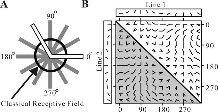
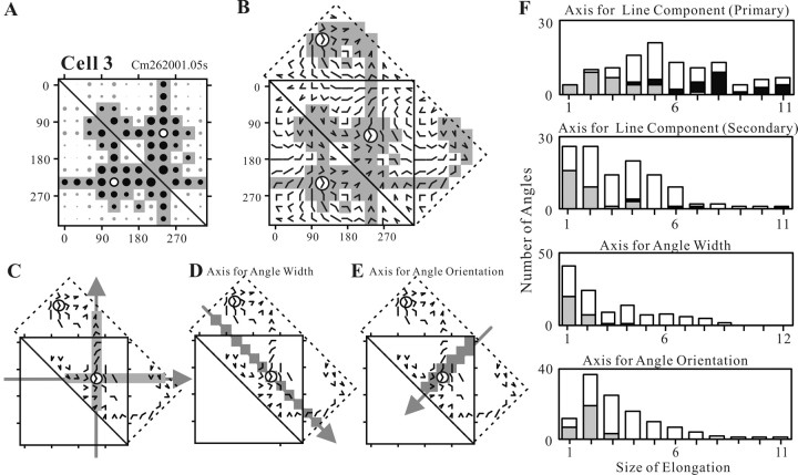
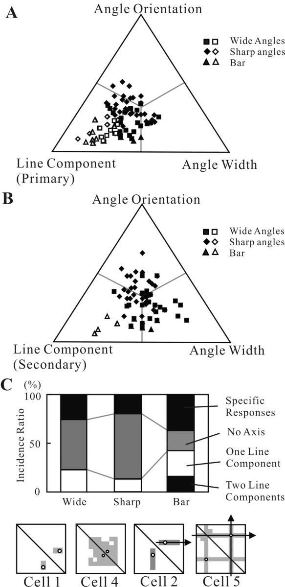
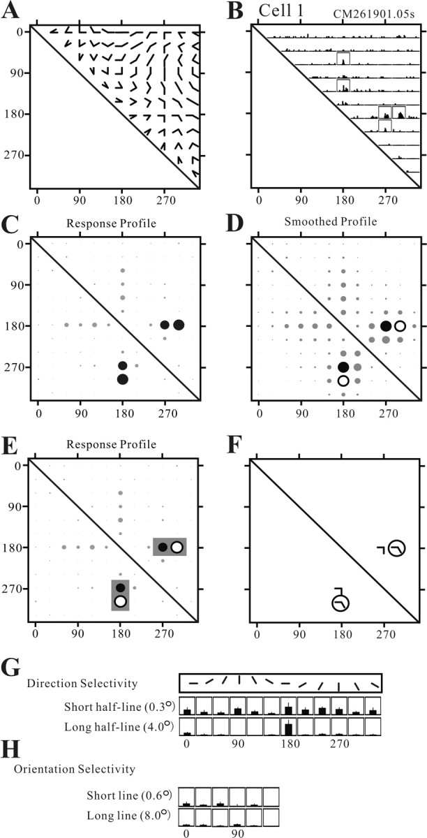
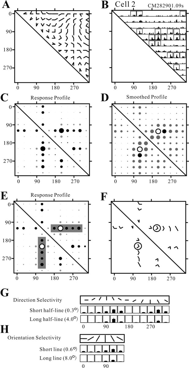
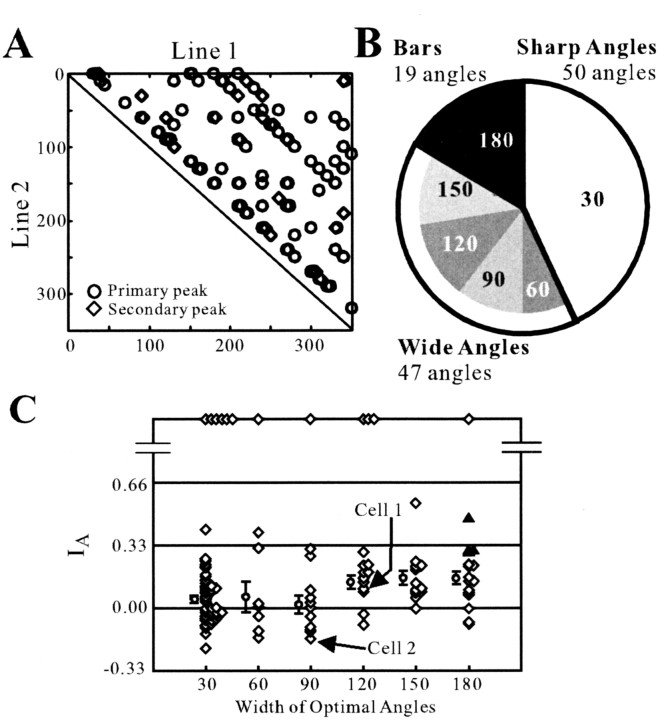
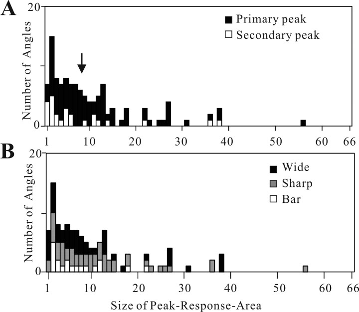
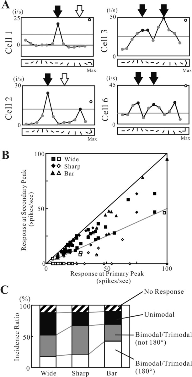
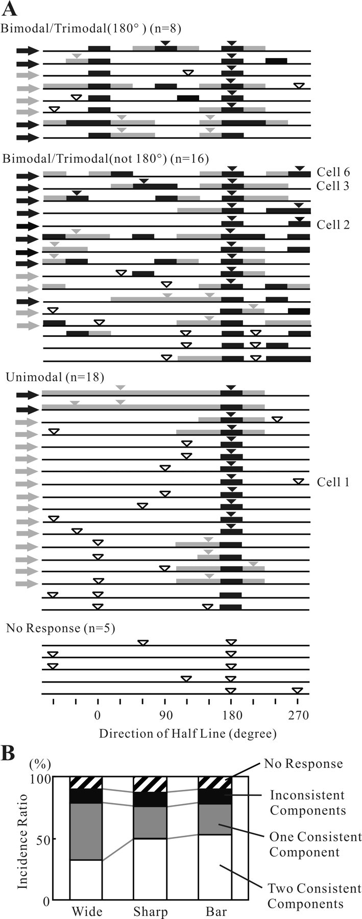
Angles and junctions embedded within contours are important features to represent the shape of objects. To study the neuronal basis to extract these features, we conducted extracellular recordings while two macaque monkeys performed a fixation task. Angle stimuli were the combination of two straight half-lines larger than the size of the classical receptive fields (CRFs). Each line was drawn from the center to outside the CRFs in 1 of 12 directions, so that the stimuli passed through the CRFs and formed angles at the center of the CRFs. Of 114 neurons recorded from the superficial layer of area V2, 91 neurons showed selective responses to these angle stimuli. Of these, 41 neurons (36.0%) showed selective responses to wide angles between 60 degrees and 150 degrees that were distinct from responses to straight lines or sharp angles (30 degrees ). Responses were highly selective to a particular angle in approximately one-fourth of neurons. When we tested the selectivity of the same neurons to individual half-lines, the preferred direction was more or less consistent with one or two components of the optimal angle stimuli. These results suggest that the selectivity of the neurons depends on both the combination of two components and the responses to individual components. Angle-selective V2 neurons are unlikely to be specific angle detectors, because the magnitude of their responses to the optimal angle was indistinguishable from that to the optimal half-lines. We suggest that the extraction of information of angles embedded within contour stimuli may start in area V2.

Figure 1.

A, Angle stimuli were composed of combinations of two long half-lines. An example of an angle stimulus composed of 0° and 120° half-lines is indicated by white lines. Each half-line was drawn from the center to the outside of the CRF of the recorded neuron, so that stimuli passed through the CRF and formed an angle at its center. B, Angle space representing the entire set of angle stimuli used in this study. A set of 66 angle stimuli was made by changing the orientation of the half-lines in 30° steps (illustrated at the top and left) and presented as a 12 × 12 matrix. The two half-lines were exchangeable, and the gray region of the matrix is a mirror image of the white region.

Figure 6.

Elongation of the distribution of responses in the angle space was given by the number of stimuli along the four axes centered at the optimal angle. A, Distribution of responses equal to or larger than half the maximal response (gray region) in a V2 neuron (cell 3). The format is the same as in Figure 2 E. B, Extended version of the matrix of the angle space. Note that the oblique matrix shown by the broken line contains the same angle stimuli as the original matrix. The gray region contains angle stimuli inducing responses equal to or larger than half the maximum; open circles indicate the optimal angle. C–E, The four axes centered at the optimal angle in the oblique matrix (gray region). Only stimuli inducing the responses equal to or larger than half the maximum are indicated. The extent of the elongation is given by the number of these stimuli in the gray regions. C, Axes for the line components of the optimal angle. D, Axis for the angle width of the optimal angle. E, Axis for the angle orientation of the optimal angle. F, Distribution of the extents of elongation along the four axes for 116 optimal angles. For the horizontal–vertical axes, the larger axis is referred to as the primary axis, and the smaller is referred to as the secondary axis. The black column represents the optimal angles in which the extent of elongation met the criteria for axis of elongation (see Results). The gray column represents those in which the extent of elongation within the peak response area was less than three along all four axes.

Figure 7.

A, Comparison of the extent of elongation along three axes representing the primary line components, angle width, and angle orientation, respectively. Individual points show the barycenter of the three values for wide angles (squares), sharp angles (diamonds), and bars (triangles). Open symbols meet the criteria of the axis of elongation(see Results). B, Comparison of the extent of elongation along the three axes representing the secondary line components, angle width, and angle orientation, respectively. The format is the same as in A. C, Classification of the optimal angles with respect to the presence or absence of an axis of elongation. In the “Two Line Components” class, the distribution of responses had two axes of elongation representing the two line components of the optimal angles. In the “One Line Component” class, the distribution of responses had one axis of elongation representing one line component of the optimal angles. There was no elongation in the “No Axis” class and a small peak response area in the “Specific Responses” class. The incidence ratio is shown for each category of optimal angle: wide, sharp, and bar. The insets show examples of the response profiles for each of the above four classes: the gray areas indicate the peak response area, open circles indicate the optimal angle, and the arrow indicates the axis of elongation.

Figure 2.

Angle selectivity in a V2 neuron (cell 1). A, Matrix (12 × 12) containing the 66 angle stimuli. B, Responses by cell 1 to each of the angle stimuli shown as peristimulus time histograms (PSTHs) plotted at the position corresponding to the angle stimuli in the stimulus matrix. During a 600 msec period, angle stimuli were presented for 200–400 msec. Frames around PSTHs indicate that responses were significantly greater than background responses (Kolmogorov–Smirnov test; p < 0.05). The frame height corresponds to 100 spikes per second; frame width corresponds to 600 msec. C, Response profile of the same data in B. The magnitude of the response to each angle stimulus is represented as the diameter of disks in the 12 × 12 matrix. Black disks indicate responses ≥50% of the maximum. The maximal response was 23.0 spikes per second. Note that the bottom left part is a mirror image of the top right part and that this neuron had only one preferred angle. D, Smoothed response profile of the same data. Open circles indicate responses to the preferred angle. Black disks indicate responses >80% of the maximum. The maximal response was 9.2 spikes per second. E, Response profile similar to C in which the open circle indicates the response to the preferred angle. The gray area indicates the peak response area. F, Angle stimuli that generated responses ≥50% of maximum are shown in the 12 × 12 matrix; the circle indicates the optimal angle stimulus. G, Direction profile measured with short (0.3°) and long (4.0°) half-lines. H, Orientation profile measured using short (0.6°) and long (8.0°) lines. Frame height in G and H corresponds to 30 spikes per second.

Figure 3.

Angle selectivity in another V2 neuron (cell 2). The format is the same as in Figure 2. The frame height corresponds to 50 spikes per second (B, G, H). The maximal responses were 17.0 spikes per second (C, E) and 9.5 spikes per second (D).

Figure 4.

A, Distribution of the preferred angles in the angle space. Horizontal and vertical axes indicate the exact directions of the half-line components of the preferred angle in degrees. Circles denote the primary peaks; diamonds denote the secondary peaks. B, Distribution of widths of the preferred angle stimuli. Each number within the circle indicates the width of the preferred angle in degrees. Three classes were distinguished: (1) wide angles, ranging between 60° and 150° (n = 47); (2) sharp angles of 30° (n = 50); and (3) bars corresponding to straight 180° angles (n = 19). C, Angle response index (I_A) of each neuron sorted according to the width of the optimal angles. Filled triangles represent neurons in which the maximal response to the angle stimulus was significantly different from that to the half-lines. Data points at the top of the graph indicate neurons in which a half-line was not sufficient to induce a significant response. Circles and error bars at the left of the data points indicate the average and the SEM.

Figure 5.

Distribution of the sizes of peak response areas. The downward arrow indicates the median (n = 116). The distribution was divided with respect to two sets of properties: primary or secondary peaks (A), and wide angles, sharp angles, or bars (B).

Figure 8.

Direction selectivity for half-lines. A, Direction profiles of four neurons. Line charts show the responses to individual half-lines oriented in 12 directions separated by 30°. Black dots indicate the peak responses, gray lines indicate the 50% of the maximum point, and the open circles at the right of the direction profile indicate the maximal responses to the angle stimuli. When response amplitudes next to the primary or secondary peaks were >95% of the peak response, they were regarded as parts of a broad preferred direction (e.g., secondary peak of cell 3). Arrows indicate the directions of the line components of the optimal angle, which may be consistent (black arrows) or inconsistent (white arrows) with the peak responses to half-lines. B, Relationships between response amplitudes of the primary and secondary peaks in three categories of optimal angle: wide (squares), sharp (diamonds), and bar (triangles). When only single peaks were observed, data were plotted on the horizontal axis. When no significant responses were induced by any half-lines, the data were omitted from the figure. The gray line indicates the point at which the height of the secondary peak is half that of the primary peak. Secondary peaks <50% of the maximum (open symbols) were discarded from further analysis. C, Classification of 116 optimal angles with respect to the direction selectivity to half-lines. Each class showed (1) “Bimodal/Trimodal (180°)” selectivity with two or three peaks, including a pair 180° apart; (2) “Bimodal/Trimodal” selectivity with two or three peaks, without a pair 180° apart; (3) “Unimodal” selectivity with only one peak; and (4) “No (significant) Response” to half-lines. Shown are the incidence ratios for each of the three categories of optimal angles: wide, sharp, and bar.

Figure 9.

Consistency between the direction selectivity for half-lines and components of optimal angles. A, Chart of the consistency among all neurons that preferred wide angles. Cells were divided into four groups with respect to the bimodality of the direction profile to half-lines. Each horizontal line corresponds to one optimal angle. Thick black lines represent the peak in the direction profile. Thick gray lines represent the peak regions in which response amplitudes are ≥50% of the maximum. Direction was aligned with the direction corresponding to one peak and assigned a value of 180°. Downward arrowheads indicate the directions of the line components of optimal angles; black arrowheads are consistent with the peak of the direction profile, gray arrowheads are consistent with the peak region, and white arrowheads are in consistent with peaks and peak regions. Rightward arrows at the left indicate the classification with respect to consistency; black arrows indicate that both two-line components were consistent; gray arrows indicate that only one line component was consistent. B, Classification of 116 optimal angles with respect to the consistency: (1) “Two Consistent Peaks”; (2) “One Consistent Peak”; (3) “Inconsistent Peaks”; and (4) “No (significant) Response” to half-lines. Shown are the incidence ratios for the three categories of optimal angles: wide, sharp, and bars.

Figure 10.

Control of eye position during stimulus presentation. A, CRF of a V2 neuron (cell 2). Optimal orientation was 0°. The dot indicates the center of the CRF, where angles were formed by combining two half-lines. FP indicates the fixation mark and the extent of the 1.0° × 1.0° fixation window. The axes are calibrated in degrees. B, Quantitative examination of the CRF. The location of a short (0.5°) line segment was shifted vertically and horizontally in 0.5° steps, and response magnitudes are shown as the height of the bar in each box of the 5 × 5 response matrix. The vertical line on top of each bar indicates the SEM of the response. The response matrix is superimposed on the same coordinates used in A, and the position of each box corresponds to where the stimulus was presented. The center of the matrix corresponds to the center of the CRF shown in A. Frame height corresponds to 50 spikes per second. C, D, Mean (C) and SD (D) of eye positions during the recordings of each neuron (n = 91). E, Mean eye positions during stimulus presentation in 528 trials (66 angle stimuli × 8 repetitions) in a recording session from cell 2. Gray diamonds represent trials in which the response was >50% of maximum, and black diamonds represent those in which the response was <50% of maximum. F, Differences between the mean eye positions during trials in which responses were greater than half maximum and those in which responses were less than half maximum. Axes are calibrated in degrees for all panels. The different symbols represent the two monkeys in C, D, and F. Cont., Contralateral side; Ipsi., ipsilateral side.

References

1. Allman J, Miezin F, McGuinnes E (1985) Stimulus specific responses from beyond the classical receptive field: neurophysiological mechanisms for local-global comparisons in visual neurons. Annu Rev Neurosci 8: 407–430. - PubMed
1. Anzai A, Van Essen DC (2001) Receptive field substructure of monkey V2 neurons in the orientation domain. Soc Neurosci Abstr 27: 286.5.
1. Anzai A, Van Essen DC (2002) Receptive field structure of orientation selective cells in monkey V2. Soc Neurosci Abstr 28: 720.12.
1. Bakin JS, Nakayama K, Gilbert CD (2000) Visual responses in monkey areas V1 and V2 to three-dimensional surface configurations. J Neurosci 20: 8188–8198. - PMC - PubMed
1. Barlow HB, Blakemore C, Pettigrew JD (1967) The neural mechanisms of binocular depth discrimination. J Physiol (Lond) 193: 327–342. - PMC - PubMed
Publication types
LinkOut - more resources