A comparison of sequential sampling models for two-choice reaction time

Abstract

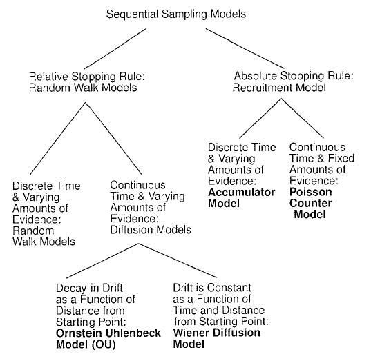
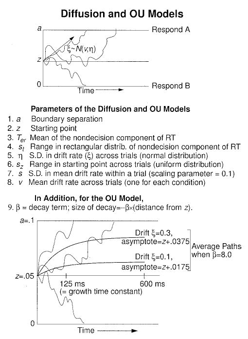
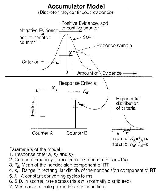
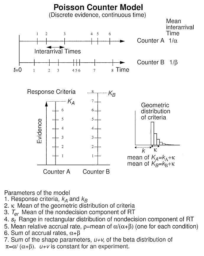
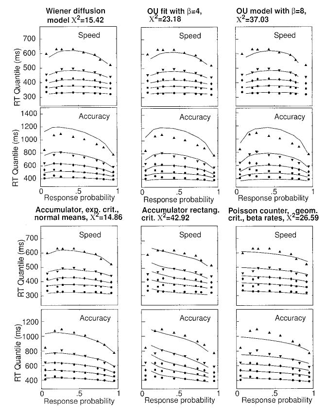
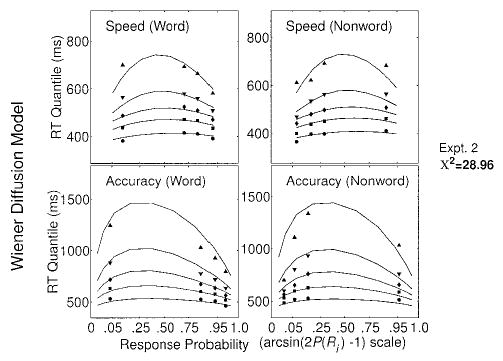
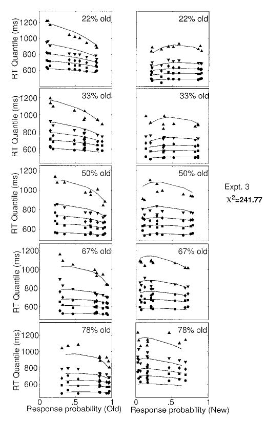
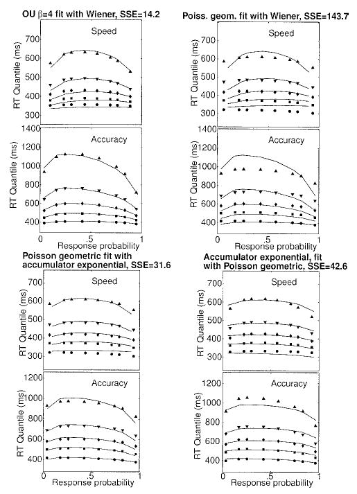
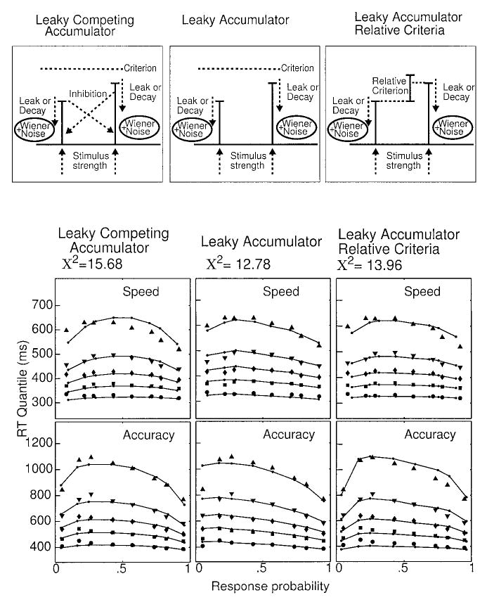
The authors evaluated 4 sequential sampling models for 2-choice decisions--the Wiener diffusion, Ornstein-Uhlenbeck (OU) diffusion, accumulator, and Poisson counter models--by fitting them to the response time (RT) distributions and accuracy data from 3 experiments. Each of the models was augmented with assumptions of variability across trials in the rate of accumulation of evidence from stimuli, the values of response criteria, and the value of base RT across trials. Although there was substantial model mimicry, empirical conditions were identified under which the models make discriminably different predictions. The best accounts of the data were provided by the Wiener diffusion model, the OU model with small-to-moderate decay, and the accumulator model with long-tailed (exponential) distributions of criteria, although the last was unable to produce error RTs shorter than correct RTs. The relationship between these models and 3 recent, neurally inspired models was also examined.

Figure 1

The relationship between the various stochastic reaction time models. The models evaluated in this article are in bold.

Figure 2

Illustration of the Wiener and Ornstein–Uhlenbeck (OU) diffusion models with a list of parameters. RT = response time; distrib. = distribution; S.D. = standard deviation.

Figure 3

Illustration of the accumulator model with a list of parameters. RT = response time; distrib. = distribution; S.D. = standard deviation.

Figure 4

Illustration of the Poisson counter model with a list of parameters. RT = response time.

Figure 5

Mapping from quantiles to response time distributions. The distances between quantiles (e.g., X and Y in the left panel) map into width of the rectangles in the histograms on the right. Prob. = probability.

Figure 6

Fits of the Wiener and Ornstein–Uhlenbeck (OU) diffusion models and the accumulator and Poisson counter model for the data from Experiment 1. The decay parameter (β) was fixed for the two OU model fits. RT = response time; exp. crit. = exponential criteria; rectang. crit. = rectangular criteria; geom. crit. = geometric criteria; ^ = .1 quantile RT; ▪ = .3 quantile RT; ♦ = .5 quantile RT; ▾ = .7 quantile RT; ▴ = .9 quantile RT.

Figure 7

Fits of the Wiener diffusion model to the data from Experiment (Expt.) 2. RT = response time; ^ = .1 quantile RT; ▪ = .3 quantile RT; ♦ = .5 quantile RT; ▾ = .7 quantile RT; ▴ = .9 quantile RT.

Figure 8

Fits of the Wiener diffusion model to the data from Experiment (Expt.) 3. RT = response time; ^ = .1 quantile RT; ▪ = .3 quantile RT;♦ = .5 quantile RT; ▾ = .7 quantile RT; ▴ = .9 quantile RT.

Figure 9

Fits of the Wiener diffusion model to predictions from the Ornstein–Uhlenbeck (OU; β = 4) and the Poisson counter models with geometrically distributed criteria, fits of the Poisson counter model with geometrically distributed criteria to the accumulator model with exponentially distributed criteria, and fits of the accumulator model with exponentially distributed criteria to the Poisson counter model with geometrically distributed criteria. Poiss. geom. = Poisson geometric; RT = response time; ^ = .1 quantile RT; ▪ = .3 quantile RT; ♦ = .5 quantile RT; ▾ = .7 quantile RT; ▴ = .9 quantile RT.

Figure 10

Illustrations of the Usher and McClelland (2001) leaky competing accumulator, the leaky accumulator, and the leaky accumulator with a relative criterion (top) and fits of these models to data from Experiment 1 (bottom). Parameters of the fit for the leaky competing accumulator were as follows: speed criterion = 1.30; accuracy criterion = 1.94; criterion range = 1.02; T_er = 276 ms; s_t = 7.3 ms; four accrual rates = .556, .676, .759, and .965; inhibition (β) = 3.49; decay constant (k) = 0.077; and standard deviation in within-trial noise (σ) = 0.675. The parameters for the leaky accumulator were as follows: speed criterion = 1.30; accuracy criterion = 1.91; criterion range = 0.372; T_er = 240 ms; s_t = 114 ms; four accrual rates = .555, .685, .780, and .994; decay constant (k) = 0.309; standard deviation in within-trial noise (s) = 0.503; and variability in drift rate across trials = 0.240. The parameters for the leaky accumulator with a relative criterion were as follows: speed criterion = 0.801; accuracy criterion = 1.34; criterion range = 0.203; T_er = 233 ms; s_t = 104 ms; four accrual rates = .555, .678, .755, and .954; decay constant (k) = 0.308; standard deviation in within-trial noise (s) = 0.627; and variability in drift rate across trials = 0.178. RT = response time; T_er = mean of the nondecision component of RT; s_t = range in rectangular distribution of nondecision component of RT; ^ = .1 quantile RT; ▪ = .3 quantile RT; ♦ = .5 quantile RT; ▾ = .7 quantile RT; ▴ = .9 quantile RT.

Figure 11

Illustration of the growth of evidence in the Ornstein–Uhlenbeck and Usher and McClelland (2001) models (top). The Usher and McClelland model would have low inhibition between counters. The bottom three panels show the hit rates and false alarm (FA) rates for repeated sampling from the asymptotic distributions of evidence. The values labeled Pr are the hit and FA rates for single samples, and the overall hit and FA rates are computed from repeated samples using the single-sample probabilities (e.g., .758 = .5/[.5 + .1586]).

Figure 12

Fits of the Wiener diffusion model to data from Experiment 2 of Van Zandt et al. (2000). RT = response time.

References

1. Ashby FG. A biased random walk model of two choice reaction times. Journal of Mathematical Psychology. 1983;27:277–297.
1. Audley RJ, Mercer A. The relation between decision time and the relative response frequency in a blue-green discrimination. British Journal of Mathematical and Statistical Psychology. 1968;21:183–192. - PubMed
1. Audley RJ, Pike AR. Some alternate stochastic models of choice. British Journal of Mathematical and Statistical Psychology. 1965;18:207–225. - PubMed
1. Buonocore A, Giorno V, Nobile AG, Ricciardi L. On the two-boundary first-crossing-time problem for diffusion processes. Journal of Applied Probability. 1990;27:102–114.
1. Burbeck SL, Luce RD. Evidence from auditory simple reaction times for both change and level detectors. Perception & Psychophysics. 1982;32:117–133. - PubMed
Publication types