Involvement of monkey inferior colliculus in spatial hearing

Abstract

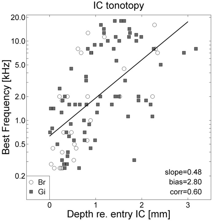
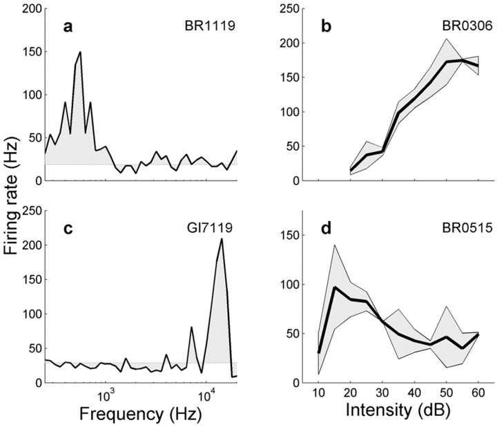
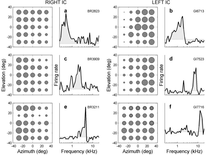
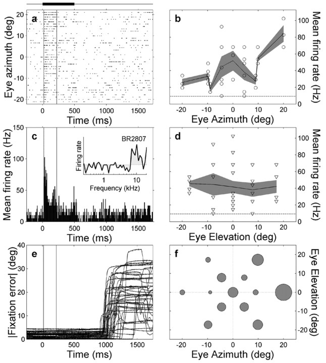
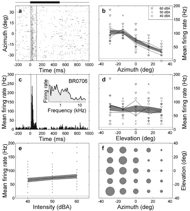
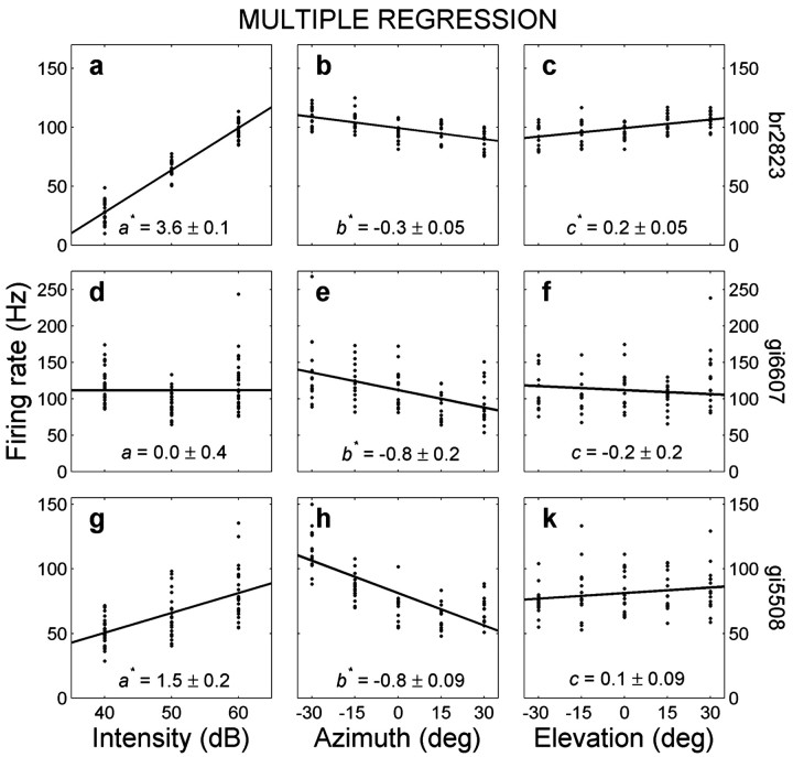
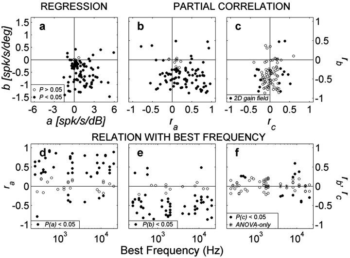
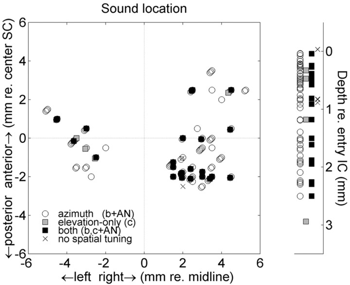
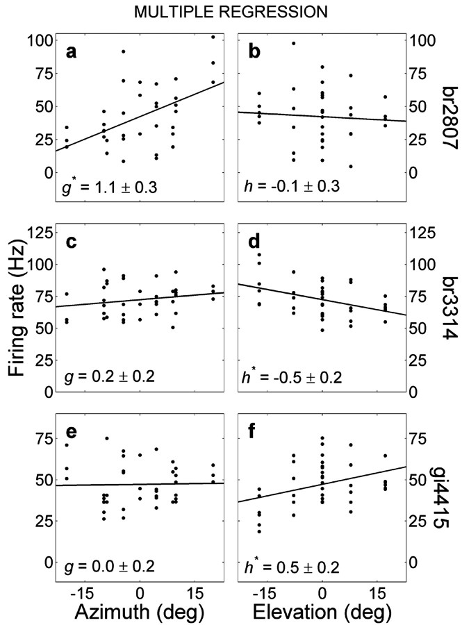
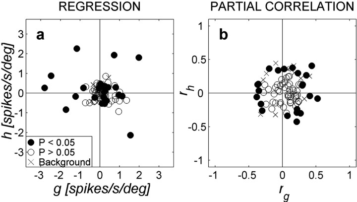
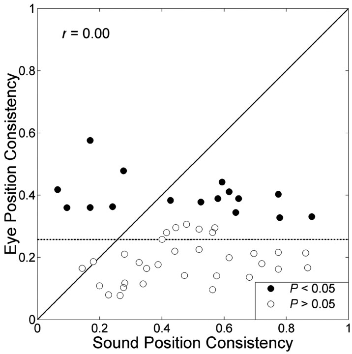
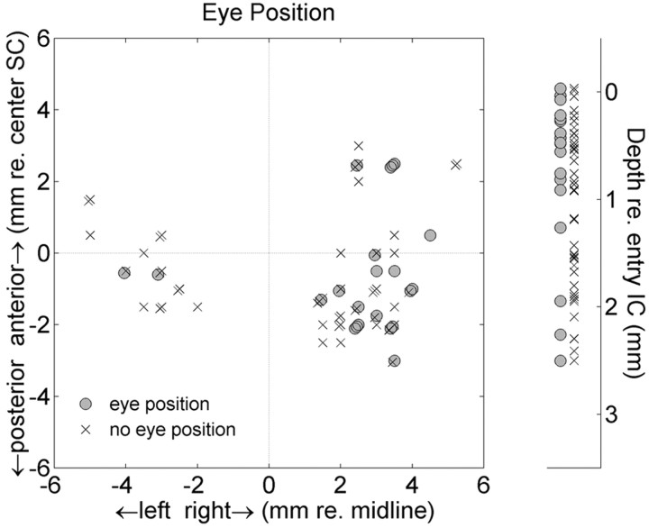
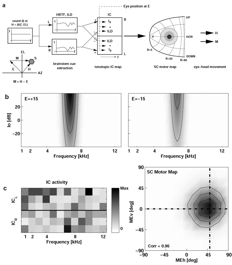
The midbrain inferior colliculus (IC) is implicated in coding sound location, but evidence from behaving primates is scarce. Here we report single-unit responses to broadband sounds that were systematically varied within the two-dimensional (2D) frontal hemifield, as well as in sound level, while monkeys fixated a central visual target. Results show that IC neurons are broadly tuned to both sound-source azimuth and level in a way that can be approximated by multiplicative, planar modulation of the firing rate of the cell. In addition, a fraction of neurons also responded to elevation. This tuning, however, was more varied: some neurons were sensitive to a specific elevation; others responded to elevation in a monotonic way. Multiple-linear regression parameters varied from cell to cell, but the only topography encountered was a dorsoventral tonotopy. In a second experiment, we presented sounds from straight ahead while monkeys fixated visual targets at different positions. We found that auditory responses in a fraction of IC cells were weakly, but systematically, modulated by 2D eye position. This modulation was absent in the spontaneous firing rates, again suggesting a multiplicative interaction of acoustic and eye-position inputs. Tuning parameters to sound frequency, location, intensity, and eye position were uncorrelated. On the basis of simulations with a simple neural network model, we suggest that the population of IC cells could encode the head-centered 2D sound location and enable a direct transformation of this signal into the eye-centered topographic motor map of the superior colliculus. Both signals are required to generate rapid eye-head orienting movements toward sounds.

Figure 2.

The BF of IC neurons increases systematically with recording depth (measured with respect to first entry in the IC). White circles, Monkey Br; gray squares, monkey Gi. Solid line, Best-fit regression of log(BF) against depth (in millimeters) for the pooled data of both monkeys (n = 105). Slope, 0.48/mm; bias, 2.80, which corresponds to 630 Hz; correlation, r = 0.60.

Figure 1.

Acoustic tuning properties of four monkey IC neurons. Left, Representative band-limited frequency tuning curves for a low-frequency (0.2-1.2 kHz) (a) and a high-frequency (8-16 kHz) (c) neuron. Response curves were averaged over three intensities (40, 50, and 60 dB) and two presentation sequences (increasing-decreasing level). Right, Monotonic (b) and non-monotonic (d) intensity tuning curves of two IC neurons. The monotonic characteristic shown in b was typical for 70% of the neurons.

Figure 4.

Six examples of neurons with low-frequency (a, b), middle-frequency (c), and high-frequency (d-f) spectral tuning curves that are sensitive to sound location with respect to head (ANOVA). Data are plotted in the same format as Figure 3f. The neurons in a and e are sensitive to both sound azimuth and elevation. The neuron in a appears to have a monotonic dependence on azimuth and elevation (i.e., 2D gain field; see also Fig. 5a-c), and the neuron in e has a non-monotonic sensitivity to elevation. The neuron in f has a monotonic sensitivity to elevation (p < 0.05) but not to azimuth (p > 0.05).

Figure 8.

Recording of neuron br2807 that is sensitive to eye position. a, Spike rasters, sorted off-line as function of eye azimuth. Vertical lines denote onset and offset of the analysis window. Note the high excitation levels for rightward eye fixations (top) and the brief post-stimulus inhibition after time 500 msec. c, PSTH and spectral tuning curve (inset) of the neuron. b, The mean firing rate of this neuron, computed within the window, increases with eye azimuth but does not vary with eye elevation (d). Dashed lines in b and d indicate mean background activity. e, Absolute eye-fixation error was small during stimulus presentation. Approximately 1 sec after stimulus on set, the monkey was rewarded, after which it made a saccadic eye movement back to the center of the oculomotor range. f, Mean firing rate (proportional to radius of filled disk; averaged over three trials) as function of 2D eye position. Note the clear trend for rightward eye positions.

Figure 3.

Illustration of response properties of IC neuron br0706 that is sensitive to sound azimuth but not to sound level. a, Spike raster is shown as function of time with respect to stimulus onset, in which each horizontal line corresponds to a single trial. Trials have been sorted off-line as function of azimuth. Thick line indicates stimulus presentation time (0-500 msec). Vertical lines denote the burst onset-offset time window within which spikes were counted (see Materials and Methods). Note systematic dependence of burst activity on sound azimuth. b, Mean firing rate (computed within the window) for three different sound levels (symbols) as function of sound-source azimuth. Note clear modulation of the activity of the cell with azimuth. Shaded band indicates mean ± 1 SD. Horizontal dashed line indicates mean spontaneous activity. c, PSTH indicates a clear onset peak (latency, 15 msec with respect to stimulus onset). Neuron is briefly inhibited after the onset peak. The neuron has a relatively broadband spectral tuning characteristic (up to ∼ 3 kHz; inset). d, Mean firing rate as function of sound elevation. Same format as in b. e, Mean firing rate as function of free-field sound level; data pooled across azimuths and elevations. f, Spatial tuning of the cell. Radius of filled circles is proportional to mean firing rate, averaged across sound levels within the particular azimuth-elevation bin.

Figure 5.

Result of the multiple linear regression analysis (Eq. 1) to dissociate the systematic sensitivity of a cell to perceived sound level (left column), sound-source azimuth (middle column), and sound elevation (right column) for three different neurons. The top neuron (br2823; a-c) is sensitive to all three parameters (see also Fig. 4a). The center neuron (gi6607; d-f) is sensitive to contralateral sound azimuth (b < 0) but not in a monotonic way to intensity or elevation. The bottom neuron (gi3918; g-k) is sensitive to both contralateral azimuth (b < 0) and sound intensity but not to elevation. Correlation coefficients between data and model are 0.96, 0.52, and 0.65, respectively. Numbers at bottom indicate mean ± SD. ^*p < 0.05 indicates a regression parameter that differs significantly from zero. Data for each variable are plotted against mean firing rate, after subtracting the weighted contributions from the other two variables.

Figure 6.

a, Distribution of regression coefficients for perceived sound level and sound azimuth for all neurons (parameters a, b of Eq. 1; pooled for both monkeys). Filled circles indicate that either parameter a or b differed significantly from zero. b, Partial correlation coefficients r_b versus r_a. The majority of neurons are tuned to contralateral locations (r_b < 0). Most neurons increase their activity with increasing sound level (r_a > 0), although a significant group (n = 9) does the reverse. Note the wide range of intensity-azimuth coefficients covered by the population. c, Partial correlations for stimulus azimuth (r_b) versus elevation (r_c). Filled circles correspond to cells with 2D spatial gain fields (i.e., both b,c ≠ 0). d-f, Bottom panels show the distribution of the partial correlation parameters r_a (left), r_b (middle), and r_c (right) as function of best frequency of each neuron for which a complete frequency tuning curve was obtained (n = 62). Filled circles correspond to significant parameter values. Note the absence of a trend.

Figure 7.

Distribution of head-centered spatial tuning characteristics of IC cells across the recording sites along lateromedial and anteroposterior coordinates (left) and along the dorsoventral (right) coordinate. Results from multiple regression (spatial parameters b, c) and ANOVA (AN) are pooled. White circles, Azimuth sensitivity; gray squares, elevation-only neurons; black squares, cells with both azimuth and elevation tuning. To enable a comparison between both monkeys, anteroposterior coordinates are given relative to the center of the overlying motor SC. Depth is measured with respect to the first entry in the IC. Spatial sensitivity is found through out the recording sites. Cells without spatial tuning (× symbols) were encountered at dorsal recording sites only.

Figure 9.

Results of multiple linear regression (Eq. 2) on eye azimuth (left; parameter g) and eye elevation (right; parameter h) for three different neurons (neuron in a and b is the same as in Fig. 8). ^* denotes a significant parameter value.

Figure 10.

Distribution of eye-position regression coefficients, shown for all 70 neurons. Filled symbols denote significant values for g and h (Eq. 2). Note that the partial correlation coefficients (b) are typically smaller than those obtained for sound location and sound level (compare with Fig. 6b). The coefficients are also unbiased for the optimal directions of the fitted eye-position vectors. × symbols correspond to cells with significant values of fitting Eq. 2 to the background activity. None of these cells coincide with the ones displaying significant eye-position modulations.

Figure 11.

Absence of a correlation between the responsiveness of a neuron to eye position and head-centered sound location, as shown here for the response consistencies to either variable (r = 0.00; dotted line indicates regression line). Black circles, Neurons with a significant modulation of eye position. White circles, Neurons without significant modulation of eye position. Head-centered sound location has a more consistent effect on cell activity than eye position, because most data points lie below the diagonal.

Figure 12.

Neurons with a significant modulation by eye position (gray circles) are widely distributed across the recording sites, without any obvious clustering. × symbols indicate cells without a significant eye-position modulation. Same format as Figure 7.

Figure 13.

a, Model of how the IC could transform tonotopic signals into an eye-centered representation of sound location in the SC. The latter emerges as a Gaussian distribution of activity with in the complex-log motor map (Robinson, 1972; Sparks, 1986). The sound has a flat spectrum, presented at random 2D locations, H, at various intensities (I). Sounds are filtered by the HRTFs (here described by elevation-dependent functions) and yield azimuth-and intensity-related inputs at the IC cells through binaural excitatory and inhibitory projections. Each IC has 12 frequency channels and, in this simulation, three cells per channel. The input bandwidth of a neuron extends between two and five channels (randomly chosen). Eye position, E, also provides a weak, modulating input to all IC cells. By training the 7200 IC-SC synapses, the network learned, in ∼2.10⁵ trials, to map all possible combinations of azimuth-elevation coordinates (range, ± 60°), eye positions (range, ± 30°), and sound intensities (range, ± 15 dB with respect to the mean) into a Gaussian population at the correct eye motor-error site within the SC motor map. b, Response field (frequency intensity) of an IC model neuron with a BF of 6 kHz, for two eye positions and H = (0 °,0 °), as determined by Eq. 3, where σ[x] = [1 + exp(-x)]^-1. Consistency of the eye-position modulation is 0.15. c, Example of a trial after training was completed. A sound (-10 dB) was presented at H = (20°,20°), with the eyes looking at E = (-30°,20°). Eye motor error is M = (50°,0°) (see inset in a, and dotted lines in right panel of c. The left panel in c shows the activity of all 72 IC cells for this trial in gray scale. IC_L, Left IC; IC_R, right IC. Lack of a simple pattern is attributable to the randomized, fixed tuning parameters of the IC cells. In this example, correlation between desired and actual activity across all 100 cells in the SC map, r = 0.96.

References

1. Aitkin L, Martin R (1990) Neurons in the inferior colliculus of cats sensitive to sound-source elevation. Hear Res 50: 97-105. - PubMed
1. Andersen RA, Roth GL, Aitkin LM, Merzenich MM (1980) The efferent projections of the central nucleus and the pericentral nucleus of the inferior colliculus in the cat. J Comp Neurol 194: 649-662. - PubMed
1. Andersen RA, Bracewell RM, Barash S, Gnadt JW, Fogassi L (1990) Eye position effects on visual, memory, and saccade-related activity in areas LIP and 7a of macaque. J Neurosci 10: 1176-1196. - PMC - PubMed
1. Andre-Deshays C, Berthoz A, Revel M (1988) Eye-head coupling in humans. I. Simultaneous recording of isolated motor units in dorsal neck muscles and horizontal eye movements. Exp Brain Res 69: 399-406. - PubMed
1. Binns KE, Grant S, Withington DJ, Keating MJ (1992) A topographic representation of auditory space in the external nucleus of the inferior colliculus of the guinea-pig. Brain Res 589: 231-242. - PubMed
Publication types
LinkOut - more resources