. 2004 May 12;24(19):4541-50.
doi: 10.1523/JNEUROSCI.4896-03.2004.

Local sensory cues and place cell directionality: additional evidence of prospective coding in the hippocampus

Affiliations

Local sensory cues and place cell directionality: additional evidence of prospective coding in the hippocampus

Francesco P Battaglia et al. J Neurosci. .

Abstract

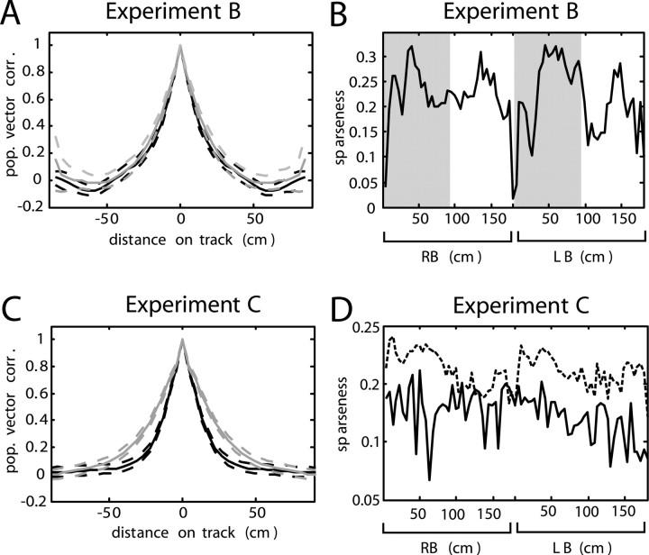
In tasks involving goal-directed, stereotyped trajectories on uniform tracks, the spatially selective activity of hippocampal principal cells depends on the animal's direction of motion. Principal cell ensemble activity while the rat moves in opposite directions through a given location is typically uncorrelated. It is shown here, with data from three experiments, that multimodal, local sensory cues can change the directional properties of CA1 pyramidal cells, inducing bidirectionality in a significant proportion of place cells. For a majority of these bidirectional place cells, place field centers in the two directions of motion were displaced relative to one another, as would be the case if the cells were representing a position in space approximately 5-10 cm ahead of the rat or if place cells were subject to strong accommodation or inhibition in the latter half of their input fields. However, place field density was not affected by the presence of local cues, but in the experimental condition with the most salient sensory cues, the CA1 population vectors in the "cue-rich" condition were sparser and changed more quickly in space than in the "cue-poor" condition. These results suggest that "view-invariant" object representations are projected to the hippocampus from lower cortical areas and can have the effect of increasing the correlation of the hippocampal input vectors in the two directions, hence decreasing the orthogonality of hippocampal output.


Figures

Figure 1.
Figure 1.
Photographs of the tracks used in experiments A-C. A, The 91 cm circular track (left) and the 130 cm circular track (right) used for experiment A (cue-rich circular tracks). B, The cue-rich–cue-poor combined linear track used for experiment B (combined cue-rich–cue-poor linear track). C, The cue-rich (top) and the cue-poor (bottom) tracks used for experiment C (independent cue-rich–cue-poor tracks).
Figure 2.
Figure 2.
Examples of bidirectional place fields and prospective shift. Six place field profiles from cells recorded in experiments B (combined cue-rich–cue-poor linear track) and C (independent cue-rich–cue-poor linear tracks) are shown. The firing rate profiles recorded during the leftbound journey (gray) and during the rightbound journey (black) are shown separately. The place fields in A-E are bidirectional (i.e., the profiles in the two directions show elevated activity in the same region of the track). A-D, Place fields showing examples of the prospective backward misalignment, a pattern observed in the majority of bidirectional place fields (supplemental Table 2, available at www.jneurosci.org) (Fig. 5). The place fields in the two directions were not perfectly aligned; rather, they were displaced backward with respect to the rat's direction.E, A bidirectional place field showing the opposite (retrospective) misalignment. F, An example of unidirectional place field. Y scale, arbitrary units.
Figure 3.
Figure 3.
Comparison of average firing rates on the two tracks of experiment C. A, Average firing rates for 64 putative pyramidal cells that exhibited place fields on both the cue-poor (x-axis) and the cue-rich (y-axis) tracks in experiment C (independent cue-rich–cue-poor tracks). There was no systematic difference in firing rate between the two environments (repeated-measures t test; not significant) and only a small correlation (r = 0.318; p < 0.05). B, Same comparison for 22 putative interneurons recorded on both tracks, showing no difference in the average firing rate between the environments (repeated-measures t test; not significant). The correlation coefficient between interneuronal firing on the cue-rich and the cue-poor track was r = 0.389. Note the difference in scales on the two graphs. Dashed lines, 45°.
Figure 4.
Figure 4.
Proportion of bidirectional place cells over the total spatially selective cells. A, The fraction of spatially selective cells that were bidirectional is shown for experiments A (two tracks), B, and C, for the cue-rich (R) and cue-poor (P) environments. Experiment A only had a cue-rich condition, and experiments B and C allow the direct comparison of the cue-rich and cue-poor conditions. B, Histogram of the overlap values for the cells recorded in the cue-rich (solid line) and cue-poor (dashed line) environments in experiments B and C.
Figure 5.
Figure 5.
Place field prospective misalignment. A, Histograms of the misalignment values between the rightbound and leftbound journey firing profiles for bidirectional place cells recorded from all cue-rich environments, yielding the largest overlap between the two profiles for all of the experiments combined. B, Histogram of the misalignment values for the bidirectional place cells recorded in the cue-poor half of experiment B. There was a preponderance of cells with positive misalignment. Note, however, that 6 of the 14 bidirectional cells in experiment B had place fields centered near the middle of the track, starting well into the cue-rich area. These place fields may be an effect of the sensory cues in the cue-rich area and of the border between the cue-rich and cue-poor areas, also a salient landmark. C, Histogram of the misalignment values for the cue-poor track in experiment C. The average misalignment was slightly negative and nonsignificantly different from zero. The slight majority of cells with a positive misalignment did not reach significance either (supplemental Table 2, available at www.jneurosci.org).
Figure 6.
Figure 6.
Population vector correlation. In each matrix, the element rij represents the Pearson correlation between the population vectors computed at location i and location j on the tracks in experiments A (cue-rich circular tracks), B (combined cue-rich–cue-poor linear track), and C (independent cue-rich–cue-poor tracks). Each matrix is divided in four quadrants. The top left quadrants represent the correlations between population vectors in the rightbound journey, and the bottom right quadrants represent the correlations between population vectors in the leftbound journey. The other two quadrants (one the transpose of the other because of matrix symmetry) represent the correlations between one population vector from the rightbound journey and one population vector from the leftbound journey. The stripe of relatively high correlation on the diagonal, highlighted by the white lines, denotes the similarity between the representations of space in the two directions, induced by the bidirectional place cells. The peaks of the correlation were not exactly on the quadrant diagonal; rather, they were shifted to one side, consistently with the backward shift of most place fields. A, B, Population vector correlation matrix for the 91 and 130 cm tracks, respectively, of experiment A. For both tracks, a high correlation stripe is evident along the diagonal of the top right-bottom left quadrants. C, Population vector correlation for experiment B. The high correlation stripe in the top right quadrant was more evident in the part of the matrix corresponding to the rich half of the track, which is consistent with the greater proportion of bidirectional place cells on that region. D, E, The population vector correlation matrices for the cue-rich (D) and the cue-poor (E) track of experiment C (independent cue-rich–cue-poor linear tracks). The stripe of elevated correlation on the leftbound versus rightbound quadrants was more marked for the cue-rich track, indicating a greater similarity between the ensemble representation of the leftbound and rightbound journeys. For both tracks, the elevated correlation stripe was shifted to one side of the diagonal, as an effect of the prevalent backward misalignments of bidirectional place fields. The correlation between same-direction representations of nearby locations (top left and bottom right quadrants on each matrix) tended to decay more slowly on the cue-poor track than on the rich track (Fig. 7). The x- and y-axes are measured in centimeters.
Figure 7.
Figure 7.
Population vector correlation (pop. vector corr.) decay and population sparseness. A, C, The mean population vector correlation as a function of the distance between the locations from which the two population vectors were recorded for experiments B (combined cue-rich–cue-poor linear track; A) and C (independent cue-rich–cue-poor tracks; C). A, The correlation decay for the cue-rich half of the maze (black) and for the cue-poor half (gray) in experiment B are displayed. The dashed line denotes the 95% bootstrap confidence interval. Population vector correlation tended to decay more slowly with distance on the cue-poor track, but the effect did not reach significance. C, The population vector correlation decay on the cue-rich track (black) and on the cue-poor track (gray) in experiment C are displayed. The correlation on the cue-poor track decayed significantly more slowly than on the rich track, showing that on the latter track the hippocampus was somewhat more capable of orthogonalizing the representation of nearby locations. B, D, The average population sparseness at each location for experiments B and C, respectively. B, There was no detectable difference in sparseness between the cue-rich (shaded) and the cue-poor halves of the track of experiment B. D, The solid line depicts the population vector sparseness for the cue-rich track. The dashed line shows the sparseness on the cue-poor track. Coding was sparser (i.e., the sparseness value was lower) on the cue-rich track. RB, Rightbound journey; LB, leftbound journey.

Similar articles

Cited by

References

    1. Barnes CA, Suster MS, Shen J, McNaughton BL (1997) Multistability of cognitive maps in the hippocampus of old rats. Nature 388: 272-275. - PubMed
    1. Battaglia FP, Sutherland GL, McNaughton BL (2002) Predictive code in bidirectional place fields. Soc Neurosci Abstr 28: 678.12.
    1. Best PJ, White AM, Minai A (2001) Spatial processing in the brain: the activity of hippocampal place cells. Annu Rev Neurosci 24: 459-486. - PubMed
    1. Bostock E, Muller RU, Kubie JL (1991) Experience-dependent modifications of hippocampal place cell firing. Hippocampus 1: 193-205. - PubMed
    1. Bower MR (2003) The neural basis of trajectory computations in rodent-posterior-parietal cortex and hippocampus. PhD thesis, University of Arizona.

Publication types