Neuronal avalanches are diverse and precise activity patterns that are stable for many hours in cortical slice cultures

Abstract

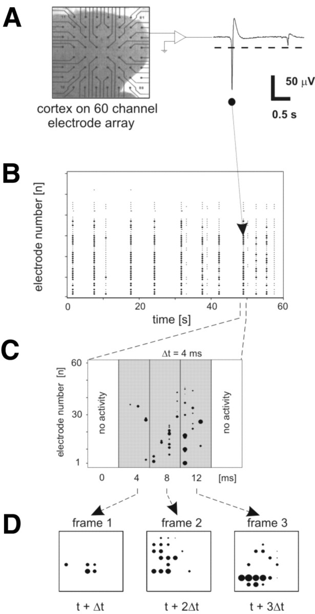
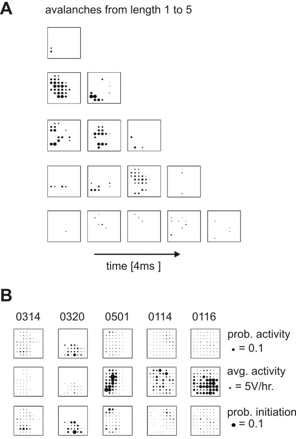
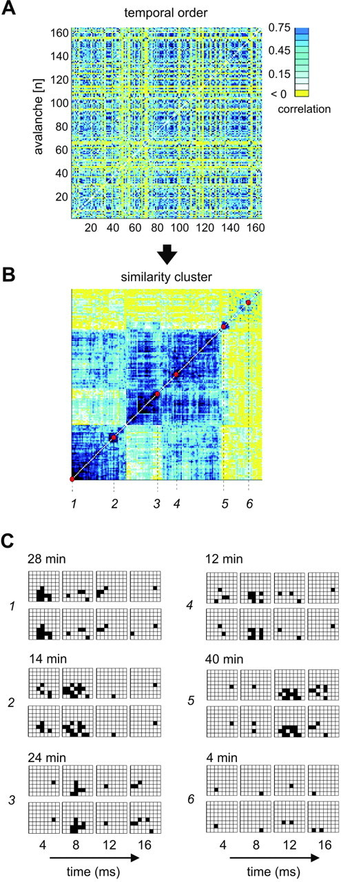
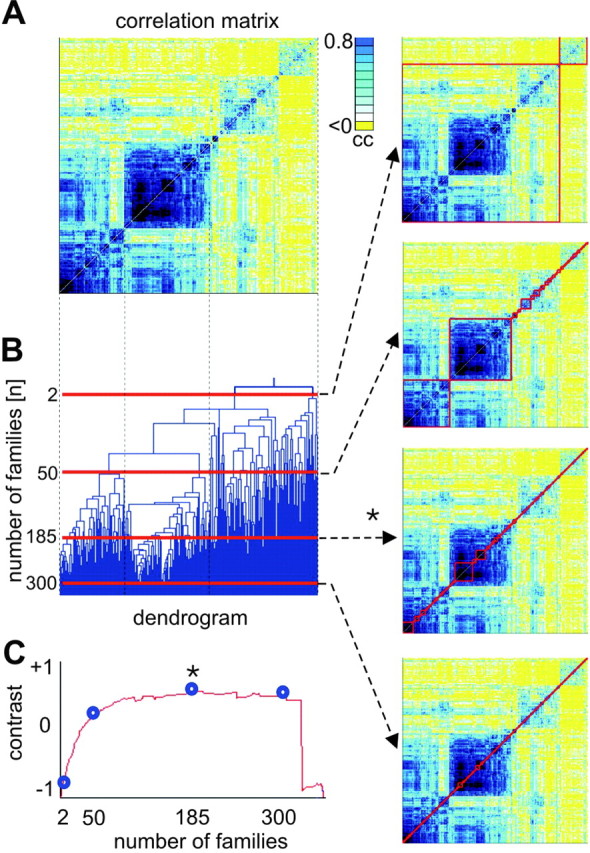
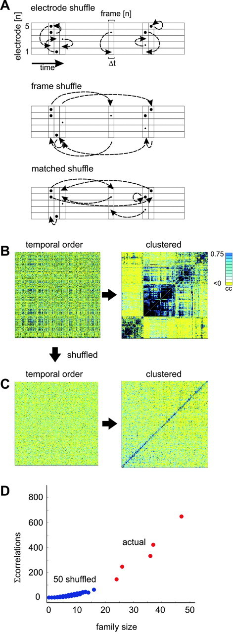
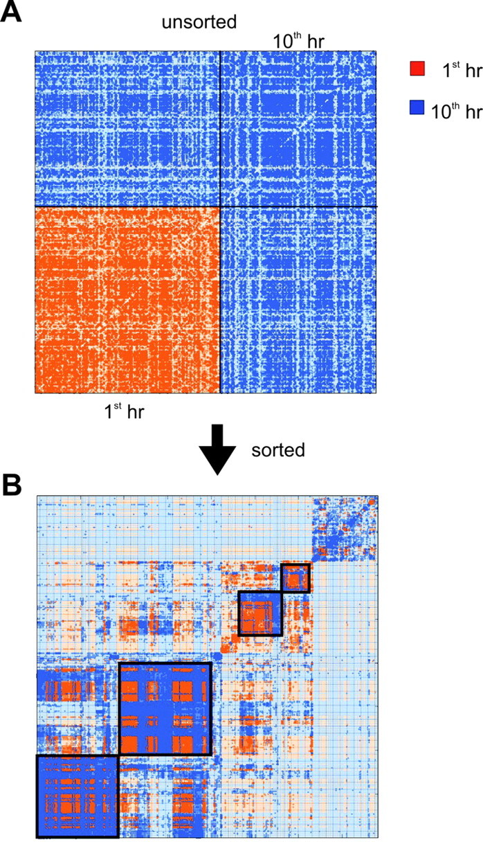
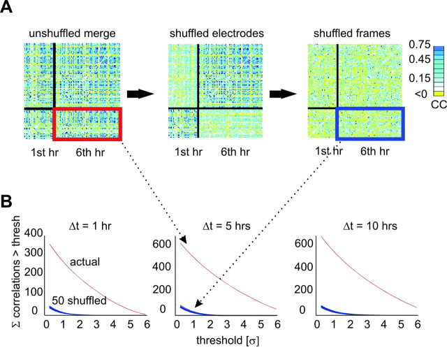
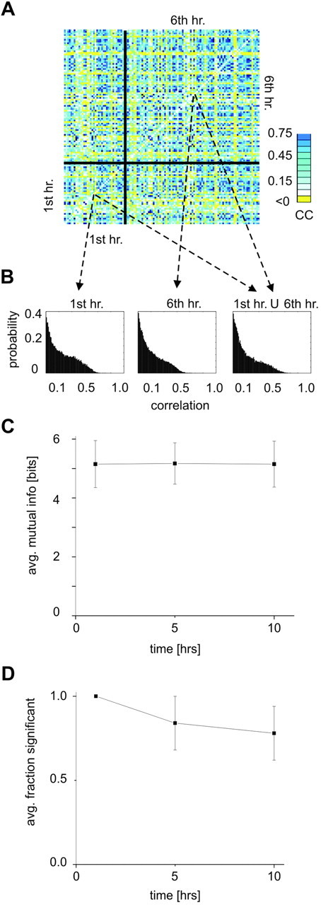
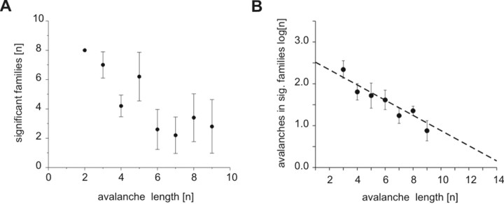
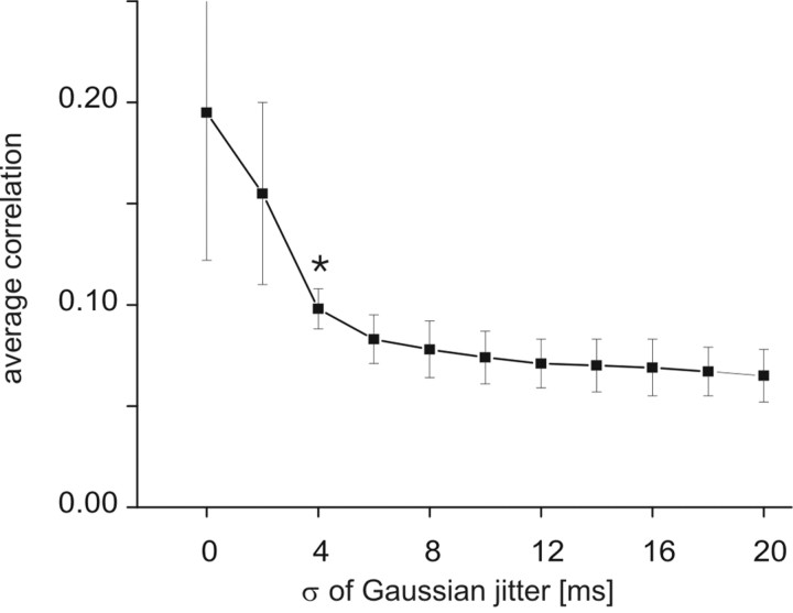
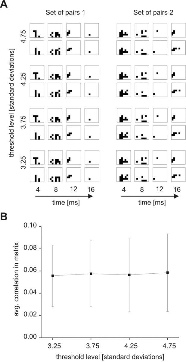
A major goal of neuroscience is to elucidate mechanisms of cortical information processing and storage. Previous work from our laboratory (Beggs and Plenz, 2003) revealed that propagation of local field potentials (LFPs) in cortical circuits could be described by the same equations that govern avalanches. Whereas modeling studies suggested that these "neuronal avalanches" were optimal for information transmission, it was not clear what role they could play in information storage. Work from numerous other laboratories has shown that cortical structures can generate reproducible spatiotemporal patterns of activity that could be used as a substrate for memory. Here, we show that although neuronal avalanches lasted only a few milliseconds, their spatiotemporal patterns were also stable and significantly repeatable even many hours later. To investigate these issues, we cultured coronal slices of rat cortex for 4 weeks on 60-channel microelectrode arrays and recorded spontaneous extracellular LFPs continuously for 10 hr. Using correlation-based clustering and a global contrast function, we found that each cortical culture spontaneously produced 4736 +/- 2769 (mean +/- SD) neuronal avalanches per hour that clustered into 30 +/- 14 statistically significant families of spatiotemporal patterns. In 10 hr of recording, over 98% of the mutual information shared by these avalanche patterns were retained. Additionally, jittering analysis revealed that the correlations between avalanches were temporally precise to within +/-4 msec. The long-term stability, diversity, and temporal precision of these avalanches indicate that they fulfill many of the requirements expected of a substrate for memory and suggest that they play a central role in both information transmission and storage within cortical networks.

Figure 1.

Multi-electrode recording of spontaneous activity in cortical slice culture. A, Left, Photo of culture grown on an MEA dish taken at 2 DIV. The interelectrode distance is 200 μm. Right, Raw activity recorded from one electrode, showing a dashed threshold line at –3 SDs. B, Raster plot shows periods of nearly synchronous activity separated by quiescent intervals of several seconds. C, Period of suprathreshold activity near the 50 sec mark in raster is binned at 4 msec, showing that activity is not exactly synchronous. Avalanches are defined as successive frames of activity with at least one electrode active. The avalanche shown spans three time bins and is preceded and terminated by a frame with no activity. D, One-dimensional arrangement of electrodes in a raster plot can be displayed as a two-dimensional frame matching the MEA grid. The activity shown in C is presented as a spatiotemporal sequence of activity on the MEA grid. In this case, an avalanche of three frames is shown. Figure 1 is reproduced from Beggs and Plenz (2003) (©2003 Society for Neuroscience).

Figure 2.

Summary of spatial activity distributions for all five networks in the current study. A, Five examples of single neuronal avalanches produced by the same culture. As before, the size of the dot indicates amplitude recorded at that electrode. Note that activity is not often wave-like and may involve large or small amplitudes. B, Statistics of activity for five different cultures. Numeric culture names are given at the column heads, whereas types of statistics and dot scales are given at the end of each row. Probability of activity (prob. activity): how likely that an electrode was to be active at any time, regardless of amplitude; average activity (avg. activity): how much a particular electrode contributed to the total activity (probability of activity times amplitude); probability of initiation (prob. initiation): how often that electrode participated in the initiation of an avalanche.

Figure 3.

Sorted correlation matrix reveals similar avalanches. A, Unsorted correlation matrix of all avalanches of length 4 recorded in 1 hr from one culture (bin width, 4 msec). Avalanches are numbered in order of appearance along the margins of the matrix. Diagonal elements have been removed for clarity. Note that blue (high correlation) and yellow (low correlation) regions are intermingled. B, Same correlation matrix as in A, now sorted in order of similarity by clustering algorithms. Note that blue regions are now concentrated along the diagonal, forming groups of avalanches with high mutual correlations. The red dots indicate regions of highly similar avalanches (numbered 1–6). C, Highly similar avalanches revealed by clustering. Each number shows a pair of avalanches that were clustered together at red dots in the sorted similarity matrix. The frames are shown as 8 × 8 grids, and suprathreshold electrodes are indicated by black squares. Differences in time of occurrence between avalanches are given in min. Note that avalanches show high spatial and temporal similarity despite occurring many minutes apart.

Figure 5.

Levels of the dendrogram correspond to different sets of families in the correlation matrix. A, Correlation matrix is positioned directly above its dendrogram. B, Dendrogram of correlation matrix (avalanche length, 4; bin width, 4 msec). At the top of the dendrogram, a single branch signifies that all avalanches are in one family. Just below this, the dendrogram divides into two branches, representing a set of two families. Branching continues further down the dendrogram until every avalanche is in its own family. The number of times each horizontal red line crosses the dendrogram indicates the number of families at that level (2, 50, 185, and 300). B, Right, Correlation matrix can be partitioned into family sets that correspond to horizontal lines on the dendrogram. Dotted arrows proceeding from each level of the dendrogram indicate how the correlation matrix is partitioned into families of avalanches at each level. Red boxes surround each family. The top matrix shows two large families, corresponding to the two branches in the dendrogram that are crossed by horizontal red line number 2. The next red line crosses 50 branches of the dendrogram, and the corresponding dotted arrow points to the matrix with 50 families surrounded by red boxes. The bottom matrices correspond to groupings with more, but smaller, families. Note that all family groupings merely represent different ways of partitioning the same correlation matrix. C, Contrast function plots contrast (compares density of correlations within red boxes to density outside of red boxes; see Materials and Methods) against the number of families, and contrast peaks at 185 families (asterisk), indicating optimum grouping into families for this matrix. The blue circles on the contrast curve correspond to the red lines drawn on the dendrogram and their corresponding groupings of families shown in matrices at right.

Figure 6.

Shuffling reveals significant families of avalanches. A, Electrode shuffling of a raster randomly permutes active electrodes within each frame but does not change the times of the frames. Any electrode that has had suprathreshold activity over the course of 1 hr is considered active. Electrode shuffling creates a data set with spatial correlations expected by chance. Frame shuffling randomly permutes times of all active frames but does not change the locations of the electrodes. This creates a data set with temporal correlations expected by chance. Matched shuffling (short for activity count matched shuffling) randomly permutes the suprathreshold activity on each electrode within the times allowed by the active frames. Note that activity on each electrode is permuted independently of other electrodes, thereby disrupting spatial correlations. Matched shuffling creates a data set with spatial and temporal correlations expected by chance, while preserving the activity rates on all electrodes and the times of active frames. B, Left, Unsorted correlation matrix of all avalanches of length 4 from actual data. Right, Same matrix now sorted to reveal clusters along the diagonal. C, Left, Unsorted correlation matrix of all avalanches of length 4 from matched shuffled data. Right, Same matrix now sorted. Note how actual data has larger blocks of high correlations along the diagonal (dark blue) than shuffled data. D, Clusters formed from actual data (red circles) have larger size and greater sum of within-cluster correlations than clusters formed from 50 sets of shuffled data (blue circles). Families of avalanches corresponding to the red circles are therefore significant at the p < 0.02 level.

Figure 7.

Coclustering reveals that avalanches are similar across time. A, Unsorted correlation matrix contains avalanches from different times. Rasters from the first and the tenth hour were merged, and all avalanches of length 4 were extracted. Correlations among avalanches from the first hour are red, all others blue. High correlations are indicated by large dots, low correlations by small dots, and negative correlations by no dots. Because correlations are presented in temporal order, red dots are to the left. B, Correlation matrix sorted in order of similarity clusters red and blue dots together into families. Families outlined by black boxes are composed of approximately equal portions of red and blue, indicating that avalanches from the first hour are similar to avalanches from the tenth hour.

Figure 4.

Examples of avalanche patterns from a single culture that are highly repeatable even after many hours. A, Avalanche pattern of length 4 was spontaneously reproduced with high similarity by the culture seven times over a period of 7.14 hr. B, Another avalanche pattern repeated six times in 6.10 hr. C, Sparse avalanche pattern reproduced four times over 7.82 hr. As before, suprathreshold electrodes are indicated by black pixels.

Figure 8.

Significant structure across many hours. A, Unsorted correlation matrices contain avalanches of length 4 from first and sixth hours. The total number of avalanches in both matrices is 120. Black lines divide the matrix into correlations within the first hour (small square, bottom left), correlations within the sixth hour (large square, top right), and interaction area that contains correlations between hours (two rectangular regions on either side of the matrix diagonal). The leftmost matrix is an unshuffled merge at which the interaction area contains many high correlations (blue pixels). The middle matrix is a merge at which data from the first hour had all electrodes randomly permuted the same way (done here merely to illustrate decoupling the hours, actual electrode shuffling was more complete, as described in Materials and Methods). This remapping preserved correlations within each hour but reduced correlations between hours, indicated by reduced blue pixels in the interaction area. The rightmost matrix is a merge at which data from both hours has had shuffled electrodes and frames. This interaction area gives correlations between the first and sixth hours expected by chance. B, Actual data are significantly different from shuffled data. The sum of correlations in the interaction area from unshuffled data (red box) plotted as a red curve against threshold for three time differences Δt. The sum of correlations in the interaction area from shuffled data (blue box) plotted as 50 blue curves against threshold for each time difference. Note that the curve for actual data are far above curves for shuffled data. Also note changes in the vertical scale. The ratio of actual correlations to shuffled correlations is fairly constant for 10 hr and remains statistically significant.

Figure 9.

The same correlations between avalanches are preserved over time. A, Merged correlation matrix from Figure 8 is shown with correlations from the first hour (bottom left box) and correlations from the sixth hour (top right box) marked out by black lines. B, Correlations that were significant are plotted as three distributions. Horizontal axes give correlation values, and vertical axes give probability of observing that correlation value. The three plots give the distribution of significant correlations observed in the first hour, the sixth hour, and the distribution produced by the union of the correlations produced by the first and sixth hours. Note the similar shapes of the distributions, indicating that the same patterns continued to correlate with each other over time. C, The average mutual information from the avalanches showed no significant decline after 10 hr. Mutual information was calculated from the entropies of the distributions of significant correlations. This graph indicates that the significant avalanches that did repeat were essentially unchanged in form over time. D, The fraction of significant correlations between avalanches from different hours declined slightly after 10 hr. Data are from avalanches of length 5 (n = 5 cultures; matched shuffling). Here, the average retention for the group was 81% after 5 hr and 73% after 10 hr. Values are represented as the fraction of what was retained after 1 hr. This graph indicates that the number of significant avalanches decreased somewhat with time.

Figure 10.

Diversity of significant families and avalanches. A, average number of significant families of avalanches plotted as a function of avalanche length. Note general decline in significant families for longer avalanches. Nevertheless, the average culture produced a total of 30 ± 14 distinct significant families, indicating that the networks could support a diversity of significant patterns. B, Log of average number of avalanches found in significant families plotted as a function of avalanche length. The dashed line is best linear fit. Again, note that the number of avalanches in significant families declines with increasing avalanche length. Still, the average significant family contained 23 avalanches, indicating that the network revisited these activity states frequently.

Figure 11.

Temporal precision of avalanches. Plot of average correlation (n = 5 cultures) against size of Gaussian jitter (see Materials and Methods). Original raster data were binned at 1 msec, and all avalanches of length 5 were extracted and used to construct correlation matrices and to obtain average correlation value. The time points within the original rasters were then jittered, and average correlation values were again extracted. Note that average correlation declines sharply with jitter, losing 49% of its original value after a jitter of 4 msec. The difference between the first two data points and the third data point was statistically significant (Tukey test; p < 0.01). The Tukey test was applied after a one-way ANOVA showed that there were significant differences between the points. This result demonstrates that the avalanches produced by spontaneous activity are temporally precise. Error bars indicate SDs.

Figure 12.

Patterns were robust with respect to thresholding. A, Pairs of avalanche patterns that were found to be similar (binary data) at different thresholds. Patterns of four frames are shown, with black pixels representing electrodes that were over threshold. A pair of similar patterns is shown at each threshold, and each column contains one set of pairs followed over different thresholds. Note that the two sets of pairs change only slightly as a function of threshold. B, Average correlation values for avalanches of length 4 remained constant over several thresholds. Binary correlation values for avalanches of length 4 from all cultures (n = 5) are shown.

References

1. Abeles M, Bergman H, Margalit E, Vaadia E (1993) Spatiotemporal firing patterns in the frontal cortex of behaving monkeys. J Neurophysiol 70: 1629–1638. - PubMed
1. Albowitz B, Kuhnt U, Ehrenreich L (1990) Optical recording of epileptiform voltage changes in the neocortical slice. Exp Brain Res 81: 241–256. - PubMed
1. Beggs JM, Plenz D (2001). Diversity and stability of elementary activity patterns that spontaneously form in isolated cortex. Soc Neurosci Abstr 27: 64.7.
1. Beggs JM, Plenz D (2003) Neuronal avalanches in neocortical circuits. J Neurosci 23: 11167–11177. - PMC - PubMed
1. Biella G, Forti M, de Curtis M (1996) Propagation of epileptiform potentials in the guinea-pig piriform cortex is sustained by associative fibres. Epilepsy Res 24: 137–146. - PubMed