Boosting accuracy of automated classification of fluorescence microscope images for location proteomics

Abstract

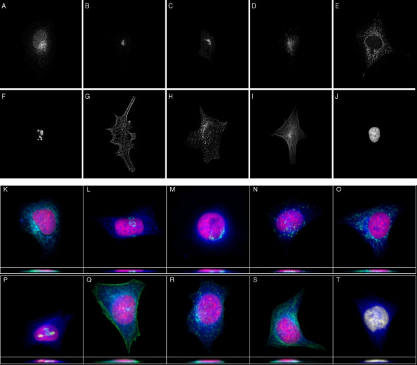
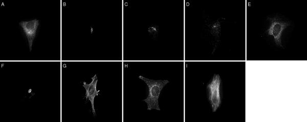
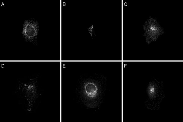
Background: Detailed knowledge of the subcellular location of each expressed protein is critical to a full understanding of its function. Fluorescence microscopy, in combination with methods for fluorescent tagging, is the most suitable current method for proteome-wide determination of subcellular location. Previous work has shown that neural network classifiers can distinguish all major protein subcellular location patterns in both 2D and 3D fluorescence microscope images. Building on these results, we evaluate here new classifiers and features to improve the recognition of protein subcellular location patterns in both 2D and 3D fluorescence microscope images.

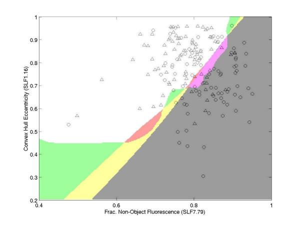
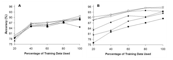
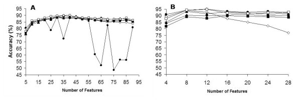
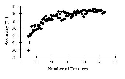
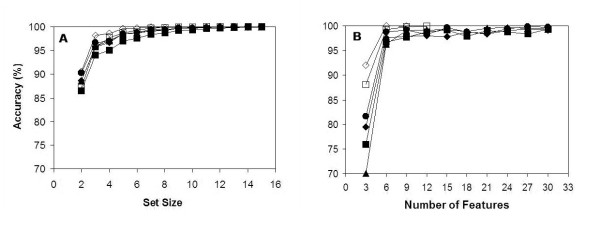
Results: We report here a thorough comparison of the performance on this problem of eight different state-of-the-art classification methods, including neural networks, support vector machines with linear, polynomial, radial basis, and exponential radial basis kernel functions, and ensemble methods such as AdaBoost, Bagging, and Mixtures-of-Experts. Ten-fold cross validation was used to evaluate each classifier with various parameters on different Subcellular Location Feature sets representing both 2D and 3D fluorescence microscope images, including new feature sets incorporating features derived from Gabor and Daubechies wavelet transforms. After optimal parameters were chosen for each of the eight classifiers, optimal majority-voting ensemble classifiers were formed for each feature set. Comparison of results for each image for all eight classifiers permits estimation of the lower bound classification error rate for each subcellular pattern, which we interpret to reflect the fraction of cells whose patterns are distorted by mitosis, cell death or acquisition errors. Overall, we obtained statistically significant improvements in classification accuracy over the best previously published results, with the overall error rate being reduced by one-third to one-half and with the average accuracy for single 2D images being higher than 90% for the first time. In particular, the classification accuracy for the easily confused endomembrane compartments (endoplasmic reticulum, Golgi, endosomes, lysosomes) was improved by 5-15%. We achieved further improvements when classification was conducted on image sets rather than on individual cell images.

Conclusions: The availability of accurate, fast, automated classification systems for protein location patterns in conjunction with high throughput fluorescence microscope imaging techniques enables a new subfield of proteomics, location proteomics. The accuracy and sensitivity of this approach represents an important alternative to low-resolution assignments by curation or sequence-based prediction.

Figure 1

Representative images of each pattern from correctly classified images using previous neural network classifiers. Ten patterns from the 2D/3D HeLa cell image collection are depicted: endoplasmic reticulum (A/K), giantin (B/L), gpp130 (C/M), LAMP2 (D/N), mitochondria (E/O), nucleolin (F/P), actin (G/Q), transferrin receptor (H/R), tubulin (I/S), and DNA (J/T). Each false color in the 3D images represents the fluorescence intensity from labeling the target protein (green), total DNA (red), and total protein (blue). Projections that are summed upon the Z or Y axis are shown. The feature sets SLF13 (2D) and SLF10 (3D) were used both for classification and for choosing a typical image.

Figure 2

Decision boundaries of various classifiers for distinguishing the patterns of two Golgi proteins. A scatterplot of the two most informative features for distinguishing images of giantin (circle) and gpp130 (triangle). These were chosen from SLF7DNA by SDA. Various classifiers were trained using just these features and maps of the class assigned to various points in the feature plane by each trained classifier were created (a zero (white) pixel corresponded to gpp130). A false color map was created by combining the decision maps for exponential-rbf kernel SVM (green), the majority-voting ensemble classifier (red), and neural networks (blue).

Figure 3

Dependence of classifier performance on amount of training data. The average performances of neural network (filled circle), SVM (open diamond), AdaBoost (filled triangle), Bagging (filled square), Mixtures-of-Experts (filled diamond), and majority-voting ensemble (open square) classifiers are shown as a function of the amount of training data given to the classifier. Average performance is defined as the average fraction of images in ten (2D) or eleven (3D) classes that were correctly classified over ten cross-validation trials. A) Results for 2D images using feature set SLF13. B) Results for 3D images using feature set SLF10.

Figure 4

Dependence of classifier performance on number of input features. The average performances of neural network (filled circle), SVM (open diamond), AdaBoost (filled triangle), Bagging (filled square), Mixtures-of-Experts (filled diamond), and majority-voting ensemble (open square) classifiers are shown as a function of the number of features used to train the classifier. Average performance is defined as the average fraction of images in ten (2D) or eleven (3D) classes that were correctly classified over ten cross-validation trials. The features in SLF7DNA (A) or SLF9 (B) were ranked in order of their ability to discriminate the classes using SDA and increasing numbers of the features were used to train classifiers.

Figure 5

Selection of feature subsets including Gabor and Daubechies features. Classifiers were trained using increasing numbers of features from the ranked list selected by SDA from either the 180-feature set including DNA features (filled circle) or the 174-feature set without DNA features (filled diamond) and performance evaluated by 10-fold cross validation. The classifiers used were the optimal majority-voting ensemble classifiers for SLF13 and SLF8 respectively (see Table 4).

Figure 6

Example 2D images that were misclassified by the original neural network classifier but could be correctly classified using the best performing ensemble classifier using SLF16. From among the images incorrectly classified by the neural network for each class, the image that was most frequently classified accurately during training of the ensemble classifier was chosen (a random choice was made in the case of ties). ER (A), giantin (B), gpp130 (C), LAMP2 (D), mitochondria (E), nucleolin (F), actin (G), transferrin receptor (H), and tubulin (I). The only DNA image that was misclassified by the original neural network classifier was also missed by the ensemble.

Figure 7

Example 2D images that could not be correctly classified by any individual classifier using feature set SLF16. The image that was most frequently classified incorrectly during training of the ensemble classifier was chosen (a random choice was made in the case of ties). ER (A), giantin (B), gpp130 (C), LAMP2 (D), mitochondria (E), and transferrin receptor (F). All images in the other classes could be correctly classified by at least one of the eight classifiers.

Figure 8

Dependence of image set classification accuracy on set size and feature set size. Panel A depicts classification accuracy for sets of images drawn from the same class. The accuracy obtained using plurality voting was averaged on 1000 random trials of image sets of various sizes drawn from each class in the test set by using the optimal majority-voting classifier for feature set SLF8 (filled square), SLF15 (filled triangle), SLF13 (filled diamond), SLF16 (filled circle), SLF14 (open square), and SLF10 (open diamond). Panel B depicts classification accuracy for reduced feature subsets using plurality voting. The accuracy obtained using plurality voting was averaged on 1000 random trials of sets of 10 images drawn from each class in the test set for various numbers of features from SLF8 (filled square), SLF15 (filled triangle), SLF13 (filled diamond), SLF16 (filled circle), SLF14 (open square), and SLF10 (open diamond).