Slow skeletal muscles of the mouse have greater initial efficiency than fast muscles but the same net efficiency

Abstract

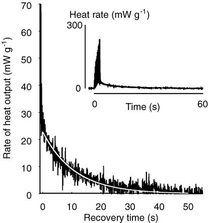
The aim of this study was to determine whether the net efficiency of mammalian muscles depends on muscle fibre type. Experiments were performed in vitro (35 degrees C) using bundles of muscle fibres from the slow-twitch soleus and fast-twitch extensor digitorum longus (EDL) muscles of the mouse. The contraction protocol consisted of 10 brief contractions, with a cyclic length change in each contraction cycle. Work output and heat production were measured and enthalpy output (work + heat) was used as the index of energy expenditure. Initial efficiency was defined as the ratio of work output to enthalpy output during the first 1 s of activity. Net efficiency was defined as the ratio of the total work produced in all the contractions to the total, suprabasal enthalpy produced in response to the contraction series, i.e. net efficiency incorporates both initial and recovery metabolism. Initial efficiency was greater in soleus (30 +/- 1%; n=6) than EDL (23 +/- 1%; n=6) but there was no difference in net efficiency between the two muscles (12.6 +/- 0.7% for soleus and 11.7 +/- 0.5% for EDL). Therefore, more recovery heat was produced per unit of initial energy expenditure in soleus than EDL. The calculated efficiency of oxidative phosphorylation was lower in soleus than EDL. The difference in recovery metabolism between soleus and EDL is unlikely to be due to effects of changes in intracellular pH on the enthalpy change associated with PCr hydrolysis. It is suggested that the functionally important specialization of slow-twitch muscle is its low rate of energy use rather than high efficiency.

Figure 1. Contraction protocol

A, an example of the strain (i.e. muscle length change) protocol used to measure ɛ_Net. Cycles were defined as starting when the first stimulus pulse in the cycle was delivered. Muscle length was altered in three phases: an isometric phase followed by constant velocity shortening at the velocity at which efficiency was maximum and then constant velocity lengthening back to the starting length. B, the time course of force output for an EDL preparation in response to the stimuli and strain shown in A. Force increased to above the shortening force during the isometric phase then during shortening declined to a steady lower value and eventually relaxed. Force output was low during lengthening. Records are from an EDL preparation (mass, 2.12 mg; length, 10.0 mm). The muscle's maximum isometric force output was 38 mN or 179 mN mm⁻².

Figure 2. Calculation of initial and net mechanical efficiency

A, initial mechanical efficiency (ɛ_I) was calculated using the first 1 s of each record, during which almost all the heat produced could be attributed to initial metabolism (i.e. PCr breakdown) and little heat was produced by recovery processes. In the example shown, from an EDL preparation contracting at 1 Hz, work and heat were produced at a high rate during the contraction (duration of each contraction, ∼0.2 s). In the interval between the first and second contractions, there was no additional heat production, consistent with the idea that no detectable recovery metabolism was occurring at this time. Enthalpy output was calculated by adding the work and heat produced and ɛ_I was calculated by dividing the amount of work produced in the first 1 s (ΔW) by the amount of enthalpy produced during the same interval (ΔH_I). The time scale indicates the time elapsed since the delivery of the first stimulus pulse. B, net mechanical efficiency (ɛ_Net) was calculated using the total work produced in all the contractions in a series (ΔW_Total) and the cumulative total of the enthalpy produced, in excess of resting metabolism, during and after the series of contractions (ΔH_Net). The records illustrated are from an EDL preparation contracting at 1 Hz.

Figure 3. Efficiency determined from relationship between power output and rate of enthalpy output

For each muscle, the relationship between power output and rate of enthalpy output was determined by performing contraction protocols at a series of contraction frequencies. The data points on each line correspond to values determined from different contraction frequencies. Initial values (▪) refer to values measured at the start of a contraction series, when recovery metabolism contributed little to the enthalpy output (see Fig. 2A). Net values (□) refer to measurements made using all the work and suprabasal enthalpy produced during and after a series of contractions (see Fig. 2B). Average power output and average enthalpy output were calculated by multiplying the average work and enthalpy output per contraction by the contraction frequency. Straight lines were fitted through the data using linear regression and initial and net efficiency values were calculated by taking the inverse of the slopes of the lines for initial values and net values, respectively. The data shown are for a soleus muscle preparation. Contraction frequencies were between 0.5 and 4.5 Hz. ɛ_I for this example was 31% and ɛ_Net was 14%.

Figure 4. Example of time course of rate of recovery heat output

Rate of heat output from a soleus preparation (black trace) following a series of 10 contractions at 3.5 Hz and at a temperature of 35°C. The time scale indicates the time elapsed since the end of the last contraction cycle. A single exponential curve was used to describe the time course of the change in recovery heat rate after the contractions ended (white line). In the example shown the rate of recovery heat immediately after the contraction series was 22.8 mW g⁻¹ and the time constant of the decline was 12.1 s. The inset shows the rate of heat output during both the contraction protocol and subsequent recovery. During the contraction series, the peak rate of heat output was greater than that during recovery, reflecting the relatively high rate of initial heat production. Preparation mass, 3.59 mg; length, 10.3 mm.

Figure 5. Initial and net efficiencies of soleus and EDL

Initial and net mechanical efficiencies were determined as illustrated in Fig. 2 using 6 muscles of each type. Initial mechanical efficiency of EDL muscles was significantly lower than that of soleus muscles. There was no significant difference in net efficiency between the two muscle types.

Figure 6. Effect of isometric duration on ɛ_Net

A, the duration of the isometric phase at the start of each contraction cycle was varied to determine whether it affected ɛ_Net. The example shows force records from a soleus with isometric durations of 25 ms (dashed line) and 50 ms (continuous line). Peak force and shortening were reduced when the isometric duration was shorter. B, ɛ_Net values for soleus (open symbols) and EDL (filled symbols) with different isometric durations. Different symbols represent data from different preparations and lines join the points for the same preparation at different isometric durations. Isometric durations were 15 and 25 ms for EDL and 25 and 50 ms for soleus preparations. There was no significant effect, for either muscle, of isometric duration of ɛ_Net.

Figure 7. Summary of kinetics of postcontractile recovery heat production

Characteristics of recovery heat production after the contraction series was completed were quantified by measuring the time constant for the decline in rate of heat production (A) and the maximum rate of recovery heat production (B). These were determined by fitting a single exponential curve through the rate of heat production data through 50 s of data after the end of the last strain cycle (Fig. 4). Symbols are mean values (± s.e.m.) for soleus (□) and EDL (▪). There was no significant effect of contraction frequency on maximum rate of recovery heat for soleus. The values for EDL varied significantly with contraction frequency. Note that, except at the lowest contraction frequencies, the rates of recovery heat are not steady state values because the duration of the contractions was too short for a steady state to be achieved. For both muscles, recovery time constant was independent of contraction frequency and the values for soleus and EDL were similar.

Figure 8. Estimated partial pressure of O₂ profiles through cylindrical muscle

The p_O2 profile through muscles calculated for steady state conditions. Profiles are shown for muscles at rest and when active. For active muscle, profiles corresponding to maximum recovery heat rates of 10 and 20 mW g⁻¹ are shown. These values span the range of measured recovery heat rates (Fig. 7A). The concentric circles (lower right) illustrate the fraction of the cross-section that would be anoxic during steady state activity giving rise to a recovery heat rate of 20 mW g⁻¹. The outer circle represents the circumference of the cylinder and the black region is the potentially anoxic area. The anoxic region corresponds to 9% of the total cross-sectional area. The average radii of soleus and EDL muscles used at 35°C in this study were 0.37 ± 0.02 and 0.40 ± 0.02 mm; a radius of 0.4 mm was used for these calculations. Other data used in the calculations: P_O2 at muscle surface, 100 kPa; diffusivity of O₂, 2.39 × 10⁻⁵ cm² atm⁻¹ min⁻¹ at 27°C (Mahler et al. 1985), adjusted to 35°C using a Q₁₀ of 1.04 (Mahler, 1978); basal metabolic rate, 1.2 mW g⁻¹ at 20°C (Crow & Kushmerick, 1982), Q₁₀ = 1.3 (Mahler, 1978).

References

1. Aickin CC, Thomas RC. An investigation of the ionic mechanism of intracellular pH regulation in mouse soleus muscle fibres. J Physiol. 1977;273:295–316. - PMC - PubMed
1. Ardevol A, Adan C, Remesar X, Fernandez-Lopez JA, Alemany M. Hind leg heat balance in obese Zucker rats during exercise. Pflugers Arch. 1998;435:454–464. - PubMed
1. Barclay CJ. Efficiency of fast- and slow-twitch muscles of the mouse performing cyclic contractions. J Exp Biol. 1994;193:65–78. - PubMed
1. Barclay CJ. Mechanical efficiency and fatigue of fast and slow muscles of the mouse. J Physiol. 1996;497:781–794. - PMC - PubMed
1. Barclay CJ. Models in which many cross-bridges attach simultaneously can explain the filament movement per ATP split during muscle contraction. Int J Biol Macromol. 2003;32:139–147. - PubMed
Publication types
LinkOut - more resources