Adaptive temporal integration of motion in direction-selective neurons in macaque visual cortex

Abstract

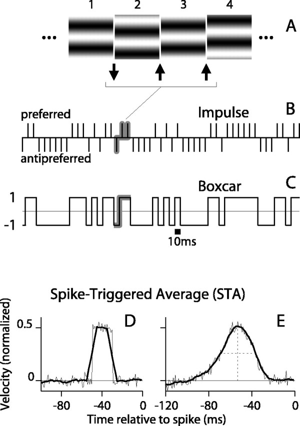
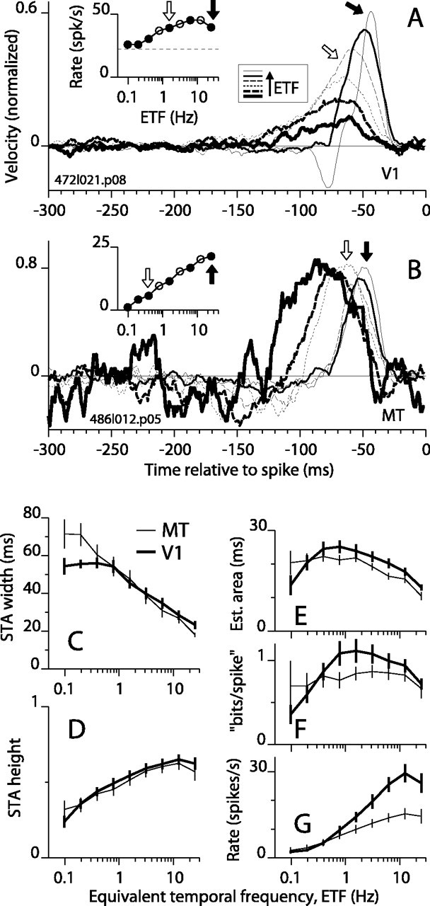
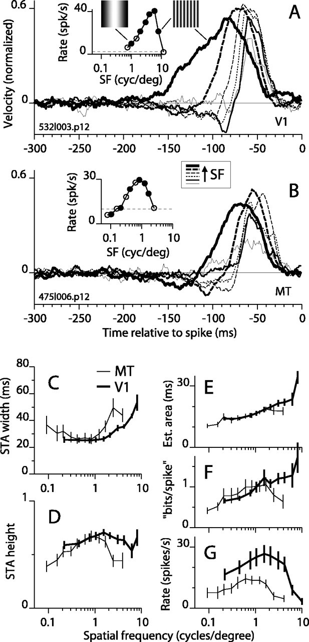
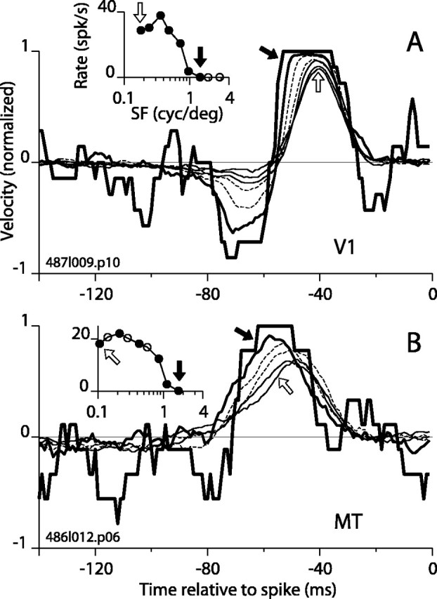
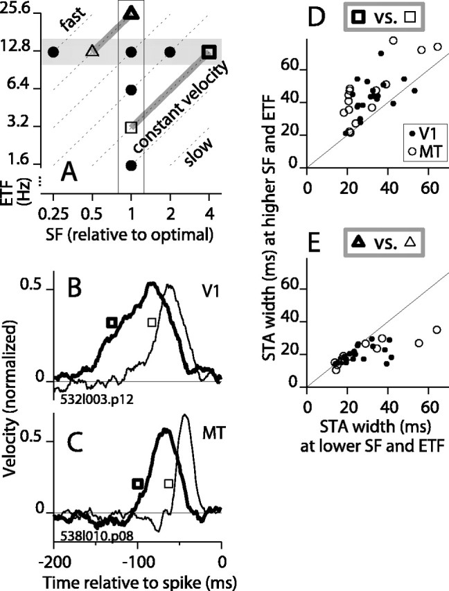
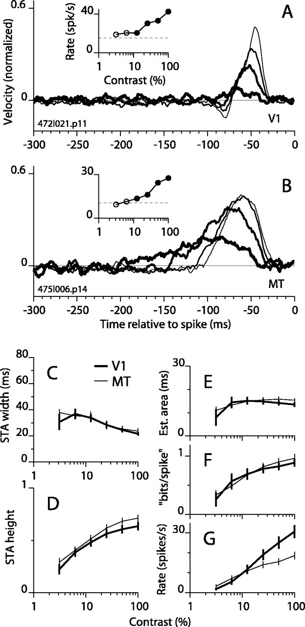
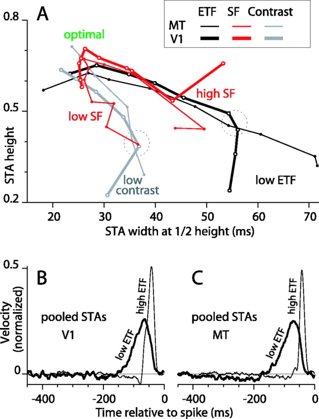
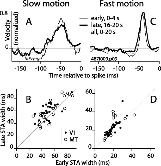
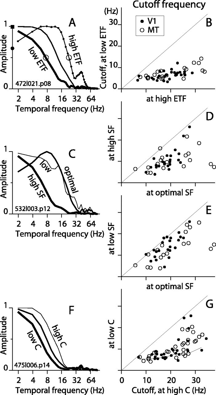
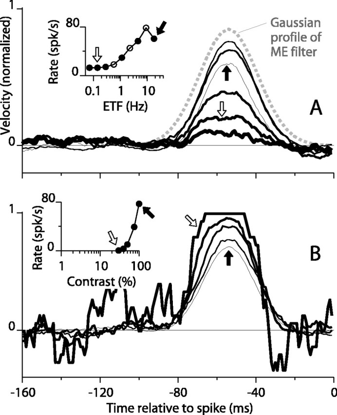
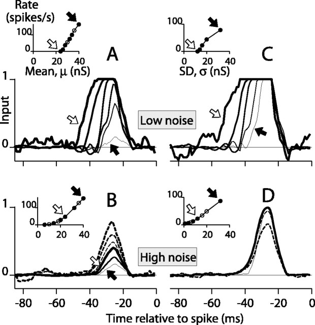
Direction-selective neurons in the primary visual cortex (V1) and the extrastriate motion area MT/V5 constitute a critical channel that links early cortical mechanisms of spatiotemporal integration to downstream signals that underlie motion perception. We studied how temporal integration in direction-selective cells depends on speed, spatial frequency (SF), and contrast using randomly moving sinusoidal gratings and spike-triggered average (STA) analysis. The window of temporal integration revealed by the STAs varied substantially with stimulus parameters, extending farther back in time for slow motion, high SF, and low contrast. At low speeds and high SF, STA peaks were larger, indicating that a single spike often conveyed more information about the stimulus under conditions in which the mean firing rate was very low. The observed trends were similar in V1 and MT and offer a physiological correlate for a large body of psychophysical data on temporal integration. We applied the same visual stimuli to a model of motion detection based on oriented linear filters (a motion energy model) that incorporated an integrate-and-fire mechanism and found that it did not account for the neuronal data. Our results show that cortical motion processing in V1 and in MT is highly nonlinear and stimulus dependent. They cast considerable doubt on the ability of simple oriented filter models to account for the output of direction-selective neurons in a general manner. Finally, they suggest that spike rate tuning functions may miss important aspects of the neural coding of motion for stimulus conditions that evoke low firing rates.

Figure 1.

The random motion stimulus and the computation of the STA. A, A sequence of four frames of the visual stimulus in which the optimal grating is shifted by 90° of phase in either the preferred (upward; up arrows) or antipreferred (downward; down arrow) direction between frames. B, The impulse representation of a 500 msec segment of stimulus is shown. The amplitude and sign of the impulses represent the size and direction of the motion (the displacement of the grating) between frames. C, The boxcar representation of the same stimulus segment takes the value 1 or -1 if the most recent movement was preferred or antipreferred, respectively. It can be constructed by convolving the function in B with a 10 msec wide boxcar. D, STAs were computed for spike trains from a model with a square window of temporal integration of duration 20 msec. The STA (thick line) computed from the boxcar stimulus was smoother than that (thin line) computed from the impulse stimulus. E, STAs computed for neuronal data. The STA (thick line) computed from the boxcar stimulus is smoother and virtually no different in shape than that (thin line) computed from the impulse stimulus.

Figure 2.

STAs as a function of stimulus ETF. A, STAs for six ETFs are plotted for an example V1 complex DS cell. In the inset, the mean firing rate is plotted for all nine ETF values tested, and the dashed line shows the spontaneous rate. In the main panel, STAs are shown only for the solid points in the inset. The arrows mark corresponding points and STA curves. The line style legend (square box) shows the progression from low to high ETF. B, STAs formatted as in A are shown for an example MT cell. Here and in A, STAs are wider for slower motion (i.e., lower ETF). C, The average width at half-height of the STA peak is plotted against ETF for 31 V1 cells and 21 MT cells. The error bars show SEM. D, The average height of the STA peak is plotted against ETF. E, The average of the product, height × width, is plotted against ETF. F, The asymptotic value of the mutual information between the stimulus and the response (calculated from the STA) in a 1 msec bin was divided by the bin width, and this measure was then divided by spike rate (see Materials and Methods). G, The mean firing rate in excess of the spontaneous rate is plotted against ETF.

Figure 3.

STAs as a function of grating SF. The format is the same as in Figure 2, except that SF is changing. A, STAs and firing rate for an example V1 cell. The icons in the spike rate inset show the visual stimuli drawn to scale for the lowest and highest (left and right, respectively) SFs that had STA peaks above the noise. High SF consistently yielded broad STAs (thickest line). The legend box between A and B shows the sequence of line styles from low to high SF. The optimal SF for drifting gratings (3 cycles/degree) corresponds to the short-dashed line. B, STAs and firing rate for an example MT cell. The optimal SF for drifting gratings corresponds to the thin long-dashed line. C-G, Same format as Figure 2, except the horizontal axis is SF. The actual SF values tested for each cell were typically not exactly those indicated by the points plotted here. The x coordinates used here are the average SF values for all points that fell in a cluster. The error bars show SEM.

Figure 4.

Single spikes can encode motion of high SF targets with certainty. A, For a V1 complex DS cell, seven STAs are shown for values of SF ranging from low (thin solid lines) to medium (dashed lines) to high (thick solid lines). From low to high SF, the STAs form a progression from a smoothed triangular shape (open arrow) to a flat-topped form (filled arrow) that indicates 100% certainty (1 on the vertical axis) that motion was in the preferred direction 35-55 msec preceding a spike. The negative lobe of the STA also extends downward, signaling an antipreferred motion with 86-93% probability from 61 to 73 msec before a spike. Thus, for the high SF stimulus, a very particular and precisely timed pattern of motion (almost always a motion reversal) was required to make this cell fire. B, Similar behavior is shown for STAs for an example MT cell. The STA for the highest SF tested (filled arrow) reaches its asymptote of 1 from 50 to 62 msec before a spike.

Figure 5.

The temporal integration profile is not determined solely by stimulus velocity. A, The typical locations of stimuli in SF-TF space are plotted for our experiments in which ETF varied (white vertical band) and in which SF varied (gray horizontal band). Points are shown only for the highest five ETFs and only for SFs at full octave intervals. Diagonals are iso-velocity contours. The thick and thin open squares connected by the long gray line segment indicate, respectively, the stimulus at the highest SF and a velocity-matched stimulus at a lower SF and lower ETF. The shorter gray line segment connecting the thick and thin triangles shows a pair of velocity-matched stimuli at a faster speed. B, For a V1 cell, the STA is plotted for SF 1 cycle/degree and ETF 12.5 Hz (thick line) and SF 0.25 cycle/degree and TF 3.1 Hz (thin line). Thus, the velocity was 12.5°/sec in both cases. The thick and thin squares indicate the positions of the stimuli in the parameter space of A. C, For an MT cell, the STA is plotted for SF 4.60 cycles/degree and TF 12.5 Hz (thick line) and for SF 1.15 cycles/degree and TF 3.1 Hz (thin line). The velocity was 2.7°/sec in both cases. D, The width at half-height of the STA at the highest SF that produced a significant peak (thick square in A) is plotted against the STA width at the optimal SF tested at the same velocity (thin square in A). Nearly all points for V1 (filled circles) and MT (open circles) fell above the line. Two points for MT, one below the line and one above the line, fell outside the range shown here: (91, 113) and (115, 73). E, The STA width at the highest ETF (25 Hz) and the optimal SF (thick triangle in A) is plotted against the width at a lower ETF (typically 12.5 Hz) at the same velocity (thin triangle in A).

Figure 6.

STAs as a function of grating contrast. The format is the same as in Figure 2, except that grating contrast is changing. A, STAs and firing rate for an example V1 cell. Only four of the six contrasts tested yielded STAs with significant peaks. As contrast was reduced from 100% to 12.5% (thinnest to thickest lines), the STA peak height decreased and became slightly broader. B, STAs and firing rates for an example MT cell. As contrast was reduced, there was a substantial broadening of the STA peak in addition to a decrease in amplitude. C-G, Same format as Figure 2, except horizontal axis is contrast.

Figure 7.

The effects on the STA shape of varying motion speed (ETF), grating SF, and grating contrast are compared. A, Data from Figures 2, 3, and 6 (C, D) are replotted in a parametric space of STA height versus width. Thick lines show data for V1 and thin lines for MT. Black lines show ETF data. Gray lines show contrast data. Red lines show SF data. Data are marked by points on lines. Low ETF marks the ends of the black lines that correspond to the slowest motion. Also labeled are the low contrast ends of the gray lines and the high SF and low SF ends of the red lines. The region marked optimal corresponds to the location of STAs for fast, high-contrast, and optimal SF stimuli. B, Database averages of the STAs for all 31 V1 complex DS cells for the two lowest ETFs (thick line) and the highest ETF (thin line). This demonstrates how the temporal profile of integration of the V1 population changes with stimulus speed. C, Averages like those in B are shown for all 21 MT cells. These averaged STAs show the dramatic change in temporal integration with motion speed for the population. It also reveals a weak negative lobe (from 200 to 400 msec before a spike) that was not easily observed in individual STAs.

Figure 8.

Changes in the width of the STA peak over time during the stimulus. A, For an example V1 complex DS cell, the STA for ETF 0.4 Hz is plotted for the first 4 sec of the stimulus (thin solid line), for the 4 sec period beginning 16 sec after stimulus onset (thick line), and for the entire stimulus (dashed line). B, For each cell, the width at half-height of the STA peak for the late epoch is plotted against that for the early epoch for the lowest ETF that yielded a significant STA peak. Points for both V1 (filled circles) and MT (open circles) fell mainly above the diagonal line. C, D, The same format as A and B, except the comparison is made for fast motion (ETF 25 Hz).

Figure 9.

Characterization of STAs in the frequency domain. A, For the example V1 cell in Figure 2A, the amplitude of the FT of the STA is plotted for ETF 0.2, 3.1, and 25 Hz (thick, medium, and thin lines, respectively). The open circles mark the cutoff frequency, defined to be the frequency at which the amplitude drops to half of the maximum value. B, The cutoff frequency for low ETF is plotted against that at ETF 25 Hz for V1 and MT cells (filled and open circles, respectively). The mean cutoff values for V1 (n = 31) were 6 Hz (SD, 2) and 19 Hz (SD, 5) for low and high ETF, respectively, and for MT (n = 21) were 7 Hz (SD, 3) and 21 Hz (SD, 10). C, For the example V1 cell in Figure 3A, the FT of the STAs are plotted for three SF values: 1.0, 2.0, and 7.9 cycles/degree (thin, medium, and thick lines, respectively). D, Cutoff frequency at high SF versus optimal SF for all cells. For V1 (n = 23), the mean cutoff dropped from 19 Hz (SD, 4) at the optimal SF to 10 Hz (SD, 5) at high SF. For MT (n = 18), the mean cutoff dropped from 21 Hz (SD, 9) for optimal SFs to 10Hz (SD, 5) for high SF. E, Cutoff frequency at low SF versus optimal SF. For V1, the mean cutoff was 14 Hz (SD, 5) at lowest SF. For MT, the mean cutoff was 13 Hz (SD, 7). F, For the example MT cell in Figure 6B, the FT of the STAs are shown for contrasts 12.5, 25, and 100% (thick, medium, and thin lines, respectively). G, Cutoff frequency at low contrast versus high contrast for all cells. The mean cutoffs at high contrast were 21 Hz (SD, 7) and 22 Hz (SD, 8) for V1 (n = 26) and MT (n = 29), respectively. At low contrast, the means were 10 Hz (SD, 5) and 11 Hz (SD, 4) for V1 and MT, respectively. For comparison, the thin line plots the mean values of the points from B.

Figure 12.

The power spectrum of the temporal modulation of luminance in our stimulus is plotted as a function of ETF. For the fastest motion (ETF 25 Hz), the spectrum is flat. For slower motion, the spectrum is low-pass, and the low-frequency cutoff decreases with ETF. See Equation 19 in the Appendix.

Figure 10.

The STAs for a motion energy model change their height, but not their width, as ETF of the visual stimulus is changed. A, The same visual stimuli used in the experimental studies were input to a motion energy detector that drove an IF unit. The inset shows the mean firing rate as a function of ETF. STAs are shown in the main panel for ETFs marked by solid points in the inset. Arrows show correspondence of STAs and points in the inset. The dashed gray line plots the Gaussian function (SD, 15 msec) used to construct the linear filters for the motion detector. B, Response versus contrast for a reconfigured model in which contrast sensitivity was unrealistically low. For this regime, c_ex was 0.5 nS, and the mean of the additive noise (both n_p and n_a), was 0 (see Eqs. 11 and 12). All other parameters remained the same (see Materials and Methods). Thicker lines show STAs for lower contrast. Arrows mark correspondence between spike rates (inset) and STAs.

Figure 11.

The shapes of STAs produced by an IF model depend on the mean and SD (μ and σ) of a random input. A, STAs from the IF model (see Materials and Methods) are shown for random binary inputs for μ from 24 to 40 nS (thicker lines indicate lower μ). The average firing rate is plotted against μ in the inset, where solid circles indicate values for which STAs are shown. The arrows mark the points and STAs for the lowest and highest means. The stimulus SD was 4 nS, and σ_noise was 2 nS. B, Increasing the additive Gaussian noise (σ_noise = 20 nS) caused the STAs to become narrower than those in A. The solid lines show STAs for the same μ and σ as in A (arrows and thickness indicate correspondence). STAs for three lower values of μ, which produced no spikes in the low noise regime in A, are shown as dashed lines (thicker dashed lines show lower μ). C, STAs are plotted for stimuli at SDs from 1 to 32 nS with μ = 16 nS and low additive noise (σ_noise = 2 nS). STA peaks were wider at lower SDs (thicker lines) than at high SDs (thinner lines). Arrows show correspondence between spike rate (inset) and STAs. D, Increasing the noise (σ_noise = 16 nS) caused the STAs to become narrower than those in C. The solid lines show STAs for the same μ and σ as in C (arrows and thickness indicate correspondence). STAs for three lower values of μ, which produced no spikes in the low noise regime in C, are shown as dashed lines (thicker dashed lines show lower μ).

References

1. Adelson EH, Bergen JR (1985) Spatiotemporal energy models for the perception of motion. J Opt Soc Am [A] 2: 284-299. - PubMed
1. Albrecht DG (1995) Visual cortex neurons in monkey and cat: effect of contrast on the spatial and temporal phase transfer functions. Vis Neurosci 12: 1191-1210. - PubMed
1. Albrecht DG, Hamilton DB (1982) Striate cortex of monkey and cat: contrast response function. J Neurophysiol 48: 217-237. - PubMed
1. Albright TD, Desimone R (1987) Local precision of visuotopic organization in the middle temporal area (MT) of the macaque. Exp Brain Res 65: 582-592. - PubMed
1. Bair W, Koch C (1996) Temporal precision of spike trains in extrastriate cortex. Neural Comput 8: 1185-1202. - PubMed
Publication types
LinkOut - more resources