Optimality principles in sensorimotor control

Abstract

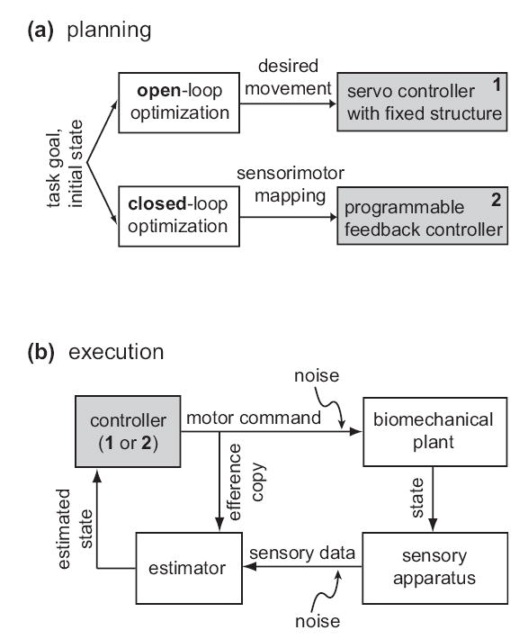
The sensorimotor system is a product of evolution, development, learning and adaptation-which work on different time scales to improve behavioral performance. Consequently, many theories of motor function are based on 'optimal performance': they quantify task goals as cost functions, and apply the sophisticated tools of optimal control theory to obtain detailed behavioral predictions. The resulting models, although not without limitations, have explained more empirical phenomena than any other class. Traditional emphasis has been on optimizing desired movement trajectories while ignoring sensory feedback. Recent work has redefined optimality in terms of feedback control laws, and focused on the mechanisms that generate behavior online. This approach has allowed researchers to fit previously unrelated concepts and observations into what may become a unified theoretical framework for interpreting motor function. At the heart of the framework is the relationship between high-level goals, and the real-time sensorimotor control strategies most suitable for accomplishing those goals.

Fig 1. Schematic illustration of open- and closed-loop optimization

(a) The optimization phase, which corresponds to planning or learning, starts with a specification of the task goal and the initial state. Both approaches yield a feedback control law, but in the case of open-loop optimization the feedback portion of the control law is predefined and not adapted to the task. (b) Either feedback controller can be used online to execute movements, although controller 2 will generally yield better performance. The estimator needs an efference copy of recent motor commands in order to compensate for sensory delays. Note that the estimator and controller are in a loop; thus they can continue to generate time-varying commands even if sensory feedback becomes unavailable. Noise is typically modeled as a property of the sensorimotor periphery, although a significant portion of it may originate in the nervous system.

Fig 2. Minimal intervention principle

Illustration of the simplest redundant task, adapted from. x₁,x₂ are two uncoupled state variables, each driven by a corresponding control signal u₁,u₂ in the presence of control-dependent noise. The task is to maintain x₁ + x₂ = target and use small controls. The optimal u₁ and u₂ are equal – to a function that depends on the task-relevant feature x₁ + x₂ but not on the individual values of x₁ and x₂. Thus u₁ and u₂ form a motor synergy. Arrows show that the optimal controls push the state vector orthogonally to the redundant direction (along which x₁ + x₂ is constant). This direction is then an uncontrolled manifold. The black ellipse is the distribution of final states, obtained by sampling the initial state from a circular Gaussian, and applying the optimal control law for one step. The gray circle is the distribution under a different control law, that tries to maintain x₁ = x₂ = target/2 by pushing the state towards the center of the plot. Such a control law can reduce variance in the redundant direction as compared to the optimal control law, but only at the expense of increased variance in the task relevant direction, as well as increased control signals (not shown). See for technical details.

Fig 3. Application of optimal feedback control to a redundant stochastic system

(a) The plant is composed of 3 point masses (X,Y,Z) and 5 actuated visco-elastic links, moving up and down in the presence of gravity. The task requires point mass X (i.e. the “end-effector”) to pass through specified targets at specified points in time. The state vector includes the lengths and velocities of links 1–3, the activation states of all actuators (modeled as low-pass filters), and the constant 1 (needed for technical reasons). The optimal feedback controller in this case is a 5x12 time-varying matrix. To understand how this matrix transforms estimated states into control signals, it was averaged over time and represented as a linear neural network (using Singular Value Decomposition). (b) Weight matrices in the neural network (color denotes sign, area denotes absolute value, ‘x’ denotes zero weight). The rows of W_S correspond to the task-relevant features being extracted; W_F are feedback gains; the columns of W_M are motor synergies. The bottom feature (with much bigger gain) extracts something closely related to end-effector position, by summing the lengths of links 1–3. The structure of the motor synergies reflects the symmetries of plant: links 3 and 5 (which act on the end-effector) are treated as a unit; links 1 and 4 (which transmit to the ground the forces generated by 3 and 5) are treated as another unit; link 2 is not actuated at all. (c) Trajectories of the point masses from 5 simulation runs. The trajectories of the end-effector are overall more repeatable than the other two point masses; also, the end-effector trajectories themselves show less variability when passing trough the targets – as observed in via-point tasks. These are both examples of variability structure arising from the minimal intervention principle. Note that the distance between the two intermediate point masses Y and Z is kept constant on average; this is an interesting emergent property due to the structure of the optimal motor synergies (which in turn reflect the structure of the plant).

Box 1. Properties of the optimal cost-to-go function

Consider the task (a) of making a pendulum swing up as quickly as possible. The pendulum is driven by a torque motor with limited output, and has to overcome gravity. Since this is a second-order system, the state vector includes the pendulum angle and angular velocity. The cost function penalizes the vertical distance away from the upright position (b) as well as the squared torque output. If we attempt to minimize this cost greedily, by always pushing up, the pendulum will never rise above some intermediate position where gravity balances the maximal torque the motor can generate. The only way to overcome gravity is to swing in one direction, and then accelerate in the opposite direction. This is similar to hitting and throwing tasks, where we have to move our arm back before accelerating it forward. The important point here is that the cost function itself does not directly suggest such a strategy. Indeed, the relationship between costs and optimal controls is rather subtle, and is mediated by another function: the optimal cost-to-go. For each state, this function tell us how much cost we will accumulate from now until the end of the movement, assuming we choose controls optimally. The optimal cost-to-go obeys a self-consistency condition known as Bellman’s optimality principle: the optimal cost-to-go at each state (c) is found by considering every possible control at that state, adding the control cost to the optimal cost-to-go for the resulting next state, and taking the minimum of these sums. The latter minimization also yields the optimal control; in (d) the color corresponds to the optimal torque as a function of the pendulum state (black: max negative; white: max positive). Plot (c) shows two optimal trajectories starting at different states. One uses the strategy of swinging back and then forward; the other goes straight to the goal because the initial velocity is sufficient to overcome gravity. Note that both trajectories in (c) are moving roughly downhill along the optimal cost-to-go surface (i.e. from light to dark). This is because, for a large class of problems, the vector of optimal control signals can be computed by taking the negative gradient of the optimal cost-to-go function, and multiplying it by a matrix that reflects plant dynamics and energy costs,. This gradient, known in control theory is the costate vector, is a vector with the same dimensionality as the state; it tells us how to change the state so as to increase the cost-to-go most rapidly. Now imagine that the costate vector is encoded by some population of neurons – which would not be surprising given its fundamental role in the computation of optimal controls. Since optimal controls are obtained from the costate via simple matrix multiplication, the activities of these neurons can directly drive muscle activation. This is reminiscent of a model of direct cortical control of muscle activation, and suggests that the costate vector is something that might be encoded in the output of primary motor cortex. What does the costate look like? As explained above, it is related to how the state varies under the action of the optimal controller; so if the state includes position and velocity, the costate might resemble a mix of velocity and acceleration. But this relationship is loose; the only general way to find the true costate is to solve the optimal control problem.

References

1. Chow CK, Jacobson DH. Studies of human locomotion via optimal programming. Math Biosciences. 1971;10:239–306.
1. Hatze H, Buys JD. Energy-optimal controls in the mammalian neuromuscular system. Biol Cybern. 1977;27:9–20. - PubMed
1. Davy DT, Audu ML. A dynamic optimization technique for predicting muscle forces in the swing phase of gait. J Biomech. 1987;20:187–201. - PubMed
1. Collins JJ. The redundant nature of locomotor optimization laws. J Biomech. 1995;28:251–267. - PubMed
1. Popovic D, Stein RB, Oguztoreli N, Lebiedowska M, Jonic S. Optimal control of walking with functional electrical stimulation: a computer simulation study. IEEE Trans Rehabil Eng. 1999;7:69–79. - PubMed
Publication types