Neighbor-constrained segmentation with level set based 3-D deformable models

Abstract

A novel method for the segmentation of multiple objects from three-dimensional (3-D) medical images using interobject constraints is presented. Our method is motivated by the observation that neighboring structures have consistent locations and shapes that provide configurations and context that aid in segmentation. We define a maximum a posteriori (MAP) estimation framework using the constraining information provided by neighboring objects to segment several objects simultaneously. We introduce a representation for the joint density function of the neighbor objects, and define joint probability distributions over the variations of the neighboring shape and position relationships of a set of training images. In order to estimate the MAP shapes of the objects, we formulate the model in terms of level set functions, and compute the associated Euler-Lagrange equations. The contours evolve both according to the neighbor prior information and the image gray level information. This method is useful in situations where there is limited interobject information as opposed to robust global atlases. In addition, we compare our level set representation of the object shape to the point distribution model. Results and validation from experiments on synthetic data and medical imagery in two-dimensional and 3-D are demonstrated.

Fig. 1

Training set: outlines of four subcortical structures—left and right amygdalae and hippocampi in 12 3-D MR brain images.

Fig. 2

The three primary modes of variance of the left amygdala, showing the mean and ± standard deviation (σ).

Fig. 3

The three primary modes of variance of the left hippocampus relative to the left amygdala (zero level set of Δ̃_2,1 + Ψ̄₁ for visualization).

Fig. 4

Outlines of left ventricles in 6 out of 16 MR training images gated and at a fixed point in the cardiac cycle.

Fig. 5

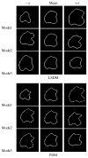
The three primary modes of variance of the left ventricle using level set (top rows) and point (bottom rows) model.

Fig. 6

Level set (black) and point model (red) based estimates of the left ventricles.

Fig. 7

Three steps in the segmentation of two shapes in a 2-D cardiac MR image (top) without and (bottom) with neighbor prior. The training set consists of 16 images. λ_i = ω_i = 0.5, i = 1, 2.

Fig. 8

Detection of eight subcortical structures (the lateral ventricles (λ = 0.8, ω = 0.2), heads of the caudate nucleus (λ= 0.3, ω = 0.7), and putamina (λ = 0.2, ω = 0.8)) in a MR brain image. (top) Results with no prior information comparing with manual segmentation. (bottom) Results with neighbor prior comparing with manual segmentation. The training set consists of 12 images.

Fig. 9

Four steps in the segmentation of the right amygdala and hippocampus. (top) Results with no prior information. (middle) Results using individual shape priors. (bottom) Results using our neighbor prior model. The training set consists of 12 brain images. λ_i = 0.1, ω_i = 0.9, i = 1, 2.

Fig. 10

Initial, middle, and final steps (top to bottom) in the segmentation of two shapes in a synthetic image. Three orthogonal slices and the 3-D surfaces are shown for each step. λ_i = 0.2, ω_i = 0.8, i = 1, 2.

Fig. 11

Initial, middle, and final steps (top to bottom) in the segmentation of four shapes in a brain image. Three orthogonal slices and the 3-D surfaces are shown for each step. λ_i = 0.1, ω_i = 0.9, i = 1, 2, 3, 4.

Fig. 12

Segmentation errors (unit: voxel) with different noise variances for synthetic image with mean intensities of objects/background: 45/65.

Fig. 13

Segmentation errors (unit:voxel) with different locations (unit:voxel) of initial seeds for synthetic image with mean intensities of objects/background: 45/65.

References

1. Kass M, Witkin A, Terzopoulos D. Snakes: Active contour models. Int J Comput Vis. 1987;1:321–331.
1. Osher S, Sethian JA. Fronts propagating with curvature-dependent speed: Algorithms based on Hamilton-Jacobi formulation. J Comp Phy. 1988;79:12–49.
1. Chan T, Vese L. Active contours without edges. IEEE Trans Image Processing. 2001 Feb;10:266–277. - PubMed
1. Cootes TF, Hill A, Taylor CJ, Haslam J. Use of active shape models for locating structures in medical images. Image Vis Computing. 1994 July;12(6):355–365.
1. Staib L, Duncan J. Boundary finding with parametrically deformable models. IEEE Trans Pattern Anal Machine Intell. 1992 Nov;14:1061–1075.