Attentional modulation of motion integration of individual neurons in the middle temporal visual area

Abstract

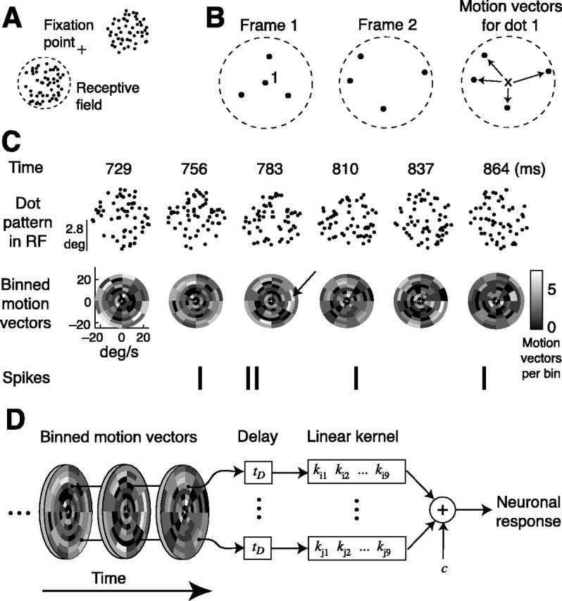
We examined how spatially directed attention affected the integration of motion in neurons of the middle temporal (MT) area of visual cortex. We recorded from single MT neurons while monkeys performed a motion detection task under two attentional states. Using 0% coherent random dot motion, we estimated the optimal linear transfer function (or kernel) between the global motion and the neuronal response. This linear kernel filtered the random dot motion across direction, speed, and time. Slightly less than one-half of the neurons produced reasonably well defined kernels that also tended to account for both the directional selectivity and responses to coherent motion of different strengths. This subpopulation of cells had faster, more transient, and more robust responses to visual stimuli than neurons with kernels that did not contain well defined regions of integration. For those neurons that had large attentional modulation and produced well defined kernels, we found attention scaled the temporal profile of the transfer function with no appreciable shift in time or change in shape. Thus, for MT neurons described by a linear transfer function, attention produced a multiplicative scaling of the temporal integration window.

Figure 1.

Description of the motion stimulus. A, The random dot stimuli consisted of two diametrically opposed patches of random dots, one of which overlapped the RF of the neuron under study. B, Example of calculating vectors between corresponding dots to describe the global motion in the stimulus. In the sequence from frame 1 to frame 2, dot 1 could have moved in one of four possible ways as illustrated by the motion vectors. There are a total of 16 motion vectors between frames 1 and 2. C, Sequence of random dots appearing in the RF of an MT neuron during an experiment. Each patch was updated every other frame on a 75 Hz monitor (every 26.6 msec). Below each patch is the polar histogram of all motion vectors between the previous and current patch. The bin location corresponds to the direction of the motion vector and the distance from the origin is the speed. The grayscale indicates the number of motion vectors per bin. Motion vectors corresponding to speeds >23.5°/sec were not included. Motion vectors were modeled as impulses occurring every 26.6 msec. The arrow indicates a strong rightward motion component occurring at 783 msec at ∼15°/sec. The corresponding recorded spike times are shown below the motion vector histograms. D, Structure of the linear kernels. Each bin of the motion vector histograms was convolved with a filter made up of nine weights (k) at 10 msec intervals. The response of the neuron was modeled as the sum of the individual filter outputs plus a constant. A variable time delay t_D was inserted to account for the latency in the neuronal response.

Figure 2.

Linear kernel for an example MT neuron. A, Kernel weights for the attend-in (left) and attend-out (right) conditions. The weights of the kernels are shown in the same polar format as the motion vectors in Figure 1C. Each time point corresponds to 96 kernel weights with linear interpolation applied between bin centers. At 40 msec, the kernel has an excitatory region (shown in white) corresponding to a motion direction of 45° and speed of 8.5°/sec. An inhibitory region (shown in black) corresponds to motion in the null direction (225°). The kernels derived from the two attentional states are nearly identical for this cell. B, Directional tuning of the neuron and linear kernel. The average neuronal response of the cell (gray filled triangles) and the predicted response of the linear kernel (black filled circles) are shown for coherent motion in different directions. The stimuli were coherent motion (50%) in each of eight directions. For the kernel, the response was calculated by convolving the linear transfer function in A with the motion vectors calculated from the random dot stimulus. The horizontal lines are the responses of the model and cell to the 0% coherent motion in the directional selectivity trials. The error bars are SEM. C, Average firing rate of a cell (gray) and linear kernel (black) to different motion coherences in the preferred direction. The open symbols correspond to the trials where the animal's attention was directed away from the RF. The horizontal lines show the neuron and the response of the model to the 0% coherent motion for the attend-in (solid) and attend-out (dashed) conditions. The average neuronal responses in B and C were calculated using the 300 msec period just before and after the coherent motion began. D, Excitatory and inhibitory temporal profiles of the linear kernel for the two attentional conditions. The excitatory temporal profiles are shown for a constant direction of 45° and a constant speed of 8.5°/sec. The inhibitory temporal profiles are for a constant direction 225° and a constant speed of 8.5°/sec. The curves are from the Gaussian function (Eq. 6) fitted to the entire kernel. Both attend-in (solid symbols) and attend-out (open symbols) profiles are shown. E, Directional tuning profile of kernels for the two attentional states. The directional profiles correspond to 40 msec and 8.5°/sec. The lines are the fitted Gaussian function.

Figure 3.

Linear kernel for a different MT neuron. The same format as in Figure 2 is shown, except as noted. D, Temporal profiles correspond to the direction of 180° (excitatory) and 0° (inhibitory) and 8.5°/sec. E, Directional tuning profiles computed at 40 msec and 8.5°/sec.

Figure 4.

Comparison of kernel S/N estimates. A, Distribution of the kernel S/N estimates for all cells. The filled bars correspond to kernels with an S/N ≥ 0.75 (good S/N). The open bars are those kernels classified as poor S/N. B, Distribution (stacked histogram) of the proportion of the average response to the coherent motion that was accounted by the linear transfer function (r_p²). The filled bars correspond to kernels with a good S/N. C, Distribution (stacked histogram) of AM in a ratiometric form. Modulation was calculated from the average response to the 0% coherent motion using an attentional index of (R_in - R_out)/(R_in + R_out), where R_in and R_out are the average response for the attend-in and attend-out conditions, respectively. The top axis shows the equivalent ratio of responses. D, Average normalized response to the onset of coherent motion (at 50% strength). E, Average normalized response to the onset of a small target located in the center of the RF. Responses are shown for cells with a good S/N (thick gray line) and a poor S/N (thin dashed black line). The error bars are SEM and, for clarity, are not shown for all points.

Figure 5.

Example of kernels with a progressively lower S/N. A, B, Example of kernels with an S/N above the 0.75 criterion and included in the analysis. C, Example of a kernel with a poor S/N and not included in the analysis.

Figure 6.

Comparison of Gaussian fit parameters (Eq. 6) for the two attentional conditions for the 44 good S/N kernels. A, Each parameter is from the fit to the kernel corresponding to the attend-in (x-axis) versus attend-out (y-axis) conditions. Kernels from each attentional condition were fit independently. Top to bottom:kernelgain (G), the center (μ_t) and width (σ_t) of the temporal integration window, and the preferred direction (μ_d) and direction tuning width (σ_d) for the attend-in and attend-out conditions. The filled symbols correspond to those neurons with good S/N kernels that also experienced ≥10% AM of the firing rate. The dashed line in each plot is unity slope. B, Distribution of AM of the Gaussian parameters. AM was computed using a ratiometric form (P_in - P_out)/(P_in + P_out) and plotted with the x-axis labeled using the corresponding ratio (P_in/P_out). For the parameters corresponding to time of peak (μ_t) and preferred direction (μ_d), the effects of attention are expressed as the difference between attend-in and attend-out. The filled bars correspond to good S/N kernels with AM of the firing rate ≥10% and the triangles correspond to the median of each parameter for the good S/N (open) and high-attention subpopulation (filled). The vertical dashed line corresponds to no AM.

Figure 7.

Average of kernels normalized by peak weight, oriented with preferred direction (μ_d) pointing up, and with temporal peak (μ_t) aligned at 0 msec and speed peak (μ_s) aligned at 8.5°/sec. Alignment of both the attend-in and attend-out kernels was based on parameters from the Gaussian fits for the attend-in condition only. A, Average population kernels from the 44 good S/N cells. Time points are relative to the alignment of the peaks. B, Average population kernels from the 20 good S/N cells that also had high AM (≥10%). C, D, Comparison of the average response predicted by the kernels with the actual average response for each subpopulation of cells. Averages were computed using the normalized responses during the 300 msec before and after the coherent motion began. The format shown is the same as that in Figure 2, B and C. The error bars are SEM.

Figure 8.

Temporal, directional, and speed profiles for the average normalized population kernels shown in Figure 7, A and B. A, Good S/N kernels. B, Good S/N plus high attention. The curves are the best fit Gaussian function (Eq. 6) using all kernel coefficients from Figure 7, A and B. The error bars are SEM.

Figure 9.

Attentional effects on the kernels and firing rates. A, AM of the amplitude (G) of the Gaussian fits versus the AM of firing rates for the 0% coherent motion. AM is expressed as a ratiometric (P_in - P_out)/(P_in + P_out), where P_in and P_out correspond to the parameter of interest for the attend-in and attend-out conditions, respectively. Shown are all good S/N kernels. The filled symbols are kernels with a high S/N ≥1.3. The dashed line is unity slope. B, The kernel scaling factor (β) expressed in an equivalent ratiometric form versus the AM of the firing rate. β was computed by nonlinearly scaling the kernel derived from the attend-out condition into the kernel corresponding to the attend-in condition. C, The kernel scaling factor (γ) expressed in an equivalent ratiometric form versus the AM of the firing rate. γ was computed by dividing the attend-in kernel SD by the attend-out kernel SD. D, Distribution of p values for the χ² test that the variance in the residual kernel, , is greater than the variance predicted by a multiplicative scaling of the noise, , or H₀: , H_A: . The filled bars correspond to those kernels with a high S/N. No kernel had a p value that was statistically significant at 0.05.

References

1. Albrecht DG, Geisler WS (1991) Motion selectivity and the contrast-response function of simple cells in the visual cortex. Vis Neurosci 7: 531-546. - PubMed
1. Albrecht DG, Hamilton DB (1982) Striate cortex of monkey and cat: contrast response function. J Neurophysiol 48: 217-237. - PubMed
1. Andersen RA, Snyder LH, Bradley DC, Xing J (1997) Multimodal representation of space in the posterior parietal cortex and its use in planning movements. Annu Rev Neurosci 20: 303-330. - PubMed
1. Bair W, Cavanaugh JR, Movshon JA (1997) Reconstructing stimulus velocity from neuronal responses in area MT. In: Advances in neural information processing systems (Mozer MC, Jordan MI, Petsche T, eds). Cambridge, MA: MIT.
1. Bair W, Cavanaugh JR, Smith MA, Movshon JA (2002) The timing of response onset and offset in macaque visual neurons. J Neurosci 22: 3189-3205. - PMC - PubMed
Publication types