3D image segmentation of deformable objects with joint shape-intensity prior models using level sets

Abstract

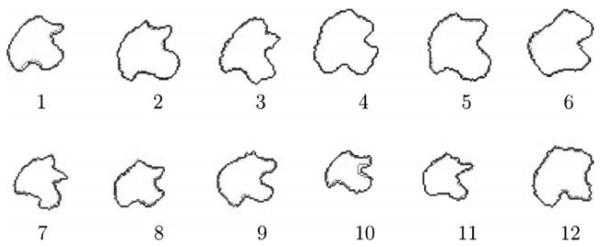
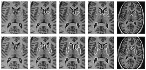
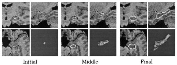
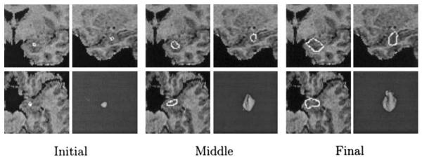
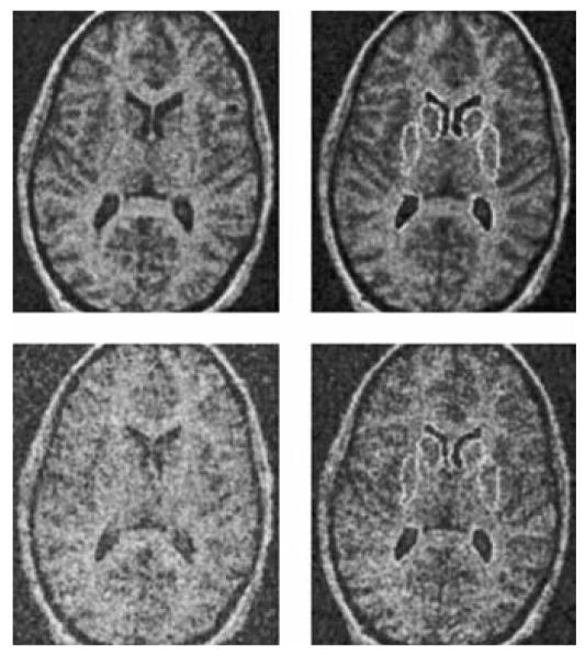
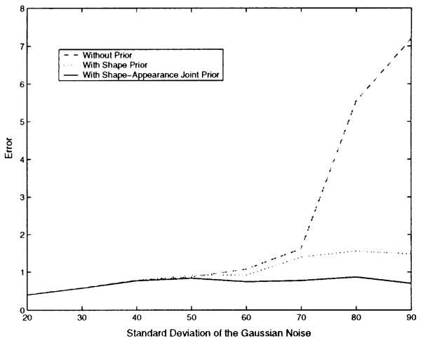
We propose a novel method for 3D image segmentation, where a Bayesian formulation, based on joint prior knowledge of the object shape and the image gray levels, along with information derived from the input image, is employed. Our method is motivated by the observation that the shape of an object and the gray level variation in an image have consistent relations that provide configurations and context that aid in segmentation. We define a maximum a posteriori (MAP) estimation model using the joint prior information of the object shape and the image gray levels to realize image segmentation. We introduce a representation for the joint density function of the object and the image gray level values, and define a joint probability distribution over the variations of the object shape and the gray levels contained in a set of training images. By estimating the MAP shape of the object, we formulate the shape-intensity model in terms of level set functions as opposed to landmark points of the object shape. In addition, we evaluate the performance of the level set representation of the object shape by comparing it with the point distribution model (PDM). We found the algorithm to be robust to noise and able to handle multidimensional data, while able to avoid the need for explicit point correspondences during the training phase. Results and validation from various experiments on 2D and 3D medical images are shown.

Fig. 1

Training set: outlines of left putamina in 12 2D MR brain images.

Fig. 2

The four primary modes of variance of the left putamen and the image gray levels, showing the mean, ±SD (σ), and ±2σ.

Fig. 3

Outlines of left ventricles in 6 out of 16 2D MR training images gated and at a fixed point in the cardiac cycle.

Fig. 4

The three primary modes of variance of the left ventricle using level set (top rows) and point (bottom rows) model, showing the mean, ±SD (σ), and ±2σ.

Fig. 5

Level set distribution model (green) and point distribution model (red) based estimates for 12 test left ventricles. The estimates are obtained from the parametric models shown in Table 1. (For interpretation of the reference to color in this figure legend, the reader is referred to the web version of this article.)

Fig. 6

Four steps of the segmentation of eight sub-cortical structures (the lateral ventricles (λ = 0.9, ω = 0.1), heads of the caudate nucleus (λ = 0.3, ω = 0.7), and putamina (λ = 0.2, ω = 0.8)) in a 2D MR brain image without prior information (top) and with shape-intensity joint prior (bottom). The training set consists of 12 MR images shown in Fig. 1.

Fig. 7

Segmentation of the left hippocampus. Three orthogonal slices and the 3D surfaces are shown for each step. The training set consists of 12 MR images λ = 0.1, ω = 0.9.

Fig. 8

Segmentation of the left amygdala. Three orthogonal slices and the 3D surfaces are shown for each step. The training set consists of 12 MR brain images. λ = 0.1, ω = 0.9.

Fig. 9

Original and segmented images with Gaussian noise of σ = 20 (top) and 40 (bottom).

Fig. 10

Segmentation errors (unit: mm) with different variances of Gaussian noise for the MR images in Fig. 6 (the mean intensities of white/gray matters: 45/65).

References

-
- Caselles V, Catte F, Coll T, Dibos F. A geometric model for active contours in image processing. Numer. Math. 1993;66:1–31.
- Caselles V, Kimmel R, Sapiro G. Geodesic active contours. Int. J. Comput. Vis. 1997;22(1):61–79.
- Chan T, Vese L. Active contours without edges. IEEE Trans. Image Process. 2001;10(2):266–277. - PubMed
- Chen Y, Tagare H, Thiruvenkadam S, Huang F, Wilson D, Gopinath KS, Briggs RW, Geiser EA. Using prior shapes in geometric active contours in a variational framework. Int. J. Comput. Vis. 2002;50(3):315–328.
- Cootes T, Beeston C, Edwards G, Taylor C. A unified framework for atlas matching using active appearance models. Inf. Process. Med. Imaging (IPMI) 1999
Publication types
MeSH terms
Grants and funding
LinkOut - more resources
Full Text Sources
Other Literature Sources