A bending mode analysis for growing microtubules: evidence for a velocity-dependent rigidity

Abstract

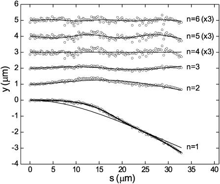
Microtubules are dynamic protein polymers that continuously switch between elongation and rapid shrinkage. They have an exceptional bending stiffness that contributes significantly to the mechanical properties of eukaryotic cells. Measurements of the persistence length of microtubules have been published since 10 years but the reported values vary over an order of magnitude without an available explanation. To precisely measure the rigidity of microtubules in their native growing state, we adapted a previously developed bending mode analysis of thermally driven shape fluctuations to the case of an elongating filament that is clamped at one end. Microtubule shapes were quantified using automated image processing, allowing for the characterization of up to five bending modes. When taken together with three other less precise measurements, our rigidity data suggest that fast-growing microtubules are less stiff than slow-growing microtubules. This would imply that care should be taken in interpreting rigidity measurements on stabilized microtubules whose growth history is not known. In addition, time analysis of bending modes showed that higher order modes relax more slowly than expected from simple hydrodynamics, possibly by the effects of internal friction within the microtubule.

FIGURE 1

Shape digitization by semiautomated image tracing. (a) Example of a partly traced image; the black line corresponds to points found by the tracing algorithm. The white horizontal bar equals 5 μm or 100 pixels. (b) Intensity line scan of the pixel column indicated by the vertical white line in Fig. 1 a. The lower left pixel in Fig. 1 a has pixel coordinates [0,0] . (c) The single period of a sine functions that was used to model the characteristic shadow-cast appearance of a microtubule. (d) Convolution results. The shaded line corresponds to the convolution of the raw data of Fig. 1 b, with the kernel of Fig. 1 c. Black lines are convolutions of nine neighboring pixel columns on the left and right side of the white line in Fig. 1 a.

FIGURE 2

(a) DIC image of an elongating microtubule. The growing plus end is on the right and the seed is on the left. The scale bar corresponds to 5 μm. (b) Same microtubule as in Fig. 2 a imaged 5 min later. The microtubule has grown out of the field of view and the shape has been changed by thermal fluctuations except for the left seed region. A digitized curve, found by automated image tracing (see Fig. 1), is superimposed on the image. The displayed coordinate system is chosen as explained in c. (c) Parameterization of microtubule shape. The path length s is chosen to be zero at the transition between the clamped (shaded) and the free (black plus white) part of the microtubule. The center of the coordinate system is located at s = 0 with the x axis along the direction of clamping. Shape can be parameterized either by y(s) or θ(s). In the experiment, only the length between s = 0 and s = (black) is analyzed. During the course of the experiment, the microtubule is growing and its full length corresponds to s = L.

FIGURE 3

Spatial part, W_n, of the first three solutions of the hydrodynamic beam equation plotted as a function of the scaled path length α = s/L. The functions are orthonormal on the interval [0,1].

FIGURE 4

Normalized contributions of full-length modes (n = 1..11) to the variance of analyzed-length modes (l = 1..6) for λ = 1.5 (a) and λ = 3 (b). Plotted contributions equal (Eq. 17).

FIGURE 5

Decomposition in modes. Plotted are raw digitized points that represent a microtubule shape at a single time point (lower curve). Only 25% of all digitized points are plotted for clarity. Mode amplitudes were calculated using Eq. 10. The thick overlaid curve is reconstituted (Eq. 11) from the first five mode amplitudes. The thin overlaid line corresponds to a reconstitution using only the first mode. Reconstitutions using only the second, third, fourth, fifth, or sixth mode are plotted with an increasing vertical offset of 1 μm (thin lines). The fourth, fifth, and sixth modes are scaled by a factor 3 for clarity. Overlaid on each nth mode curve are the raw data points with mode reconstitutions 1 until n − 1 subtracted.

FIGURE 6

Calculated mode amplitudes, ã_l, for a single microtubule (condition A, analyzed length is 34.3 μm). Data are plotted as a function of time for the first eight mode numbers. The time between data points was 6 s, and the total measurement time was 8 min.

FIGURE 7

Variance of the measured mode amplitudes, multiplied by as a function of q_l. The theoretical expectation, is plotted for our final estimates of the persistence length (Table 1). The analyzed length of the eight microtubules is given in the legend (μm). (a) Condition A. (b) Condition B.

FIGURE 8

Estimates for the persistence length for the first five modes are plotted in order of increasing filament length. Standard deviations are plotted as error bars (statistical error only). The straight line corresponds to our final estimate of the persistence length (Table 1). (a) Condition A. (b) Condition B. The first mode persistence length estimate for the microtubule with length 33.5 μm does not fit on the scale, but equals 104 mm.

FIGURE 9

Analysis of the dynamics of full-length modes. (a) Autocorrelation function (n = 2..5) of mode amplitudes that were calculated over the full length of a microtubule (L = 33.3 μm) during 24 s with 40 ms sampling time. Dashed lines are exponential fits to the initial decrease. (b) Fitted correlation time as a function of microtubule length for four full-length modes (n = 2..5). (c) Estimates for γ as a function of q_n/L. The plotted line is a fit of Eq. 20 to the data.

FIGURE 10

Persistence length estimates for five different growth conditions versus average growth velocity (see Table 3). Standard errors are plotted for the velocity and standard deviations (statistical error only) for L_p. Growth conditions with added OXS system are plotted as solid symbols and without OXS system as open symbols.

FIGURE 11

The ratio (Eq. A2), calculated for the first four mode numbers as a function of λ.

References

1. Alberts, B., A. Johnson, J. Lewis, M. Raff, K. Roberts, and P. Walter. 2002. Molecular Biology of the Cell, 4th ed. Garland Science, New York.
1. Ashkin, A. 1997. Optical trapping and manipulation of neutral particles using lasers. Proc. Natl. Acad. Sci. USA. 94:4853–4860. - PMC - PubMed
1. Cassimeris, L., D. Gard, P. T. Tran, and H. P. Erickson. 2001. XMAP215 is a long thin molecule that does not increase microtubule stiffness. J. Cell Sci. 114:3025–3033. - PubMed
1. Chretien, D., and S. D. Fuller. 2000. Microtubules switch occasionally into unfavorable configurations during elongation. J. Mol. Biol. 298:663–676. - PubMed
1. Chretien, D., F. Metoz, F. Verde, E. Karsenti, and R. H. Wade. 1992. Lattice-defects in microtubules—protofilament numbers vary within individual microtubules. J. Cell Biol. 117:1031–1040. - PMC - PubMed
LinkOut - more resources