Emergence of complex dynamics in a simple model of signaling networks

Abstract

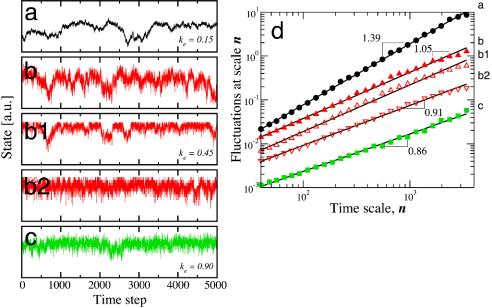
Various physical, social, and biological systems generate complex fluctuations with correlations across multiple time scales. In physiologic systems, these long-range correlations are altered with disease and aging. Such correlated fluctuations in living systems have been attributed to the interaction of multiple control systems; however, the mechanisms underlying this behavior remain unknown. Here, we show that a number of distinct classes of dynamical behaviors, including correlated fluctuations characterized by 1/f scaling of their power spectra, can emerge in networks of simple signaling units. We found that, under general conditions, complex dynamics can be generated by systems fulfilling the following two requirements, (i) a "small-world" topology and (ii) the presence of noise. Our findings support two notable conclusions. First, complex physiologic-like signals can be modeled with a minimal set of components; and second, systems fulfilling conditions i and ii are robust to some degree of degradation (i.e., they will still be able to generate 1/f dynamics).

Fig. 1.

Emergence of complex dynamics in simple signaling networks. (a) The units constituting the network, which are located on the nodes of a one-dimensional lattice, have bidirectional nearest-neighbor connections. (b) A number k_eN of additional unidirectional links is established between pairs of randomly selected units, where k_e is the mean excess connectivity and N is the number of units in the system. At time t = 0, we assign to each unit i = 1,...,N a state σ_i (0) randomly chosen from the set {0,1} and a Boolean function F_i; (Eq. 1). This Boolean function (or rule) determines the way in which the inputs are processed. Each unit effectively processes two inputs, one unit corresponding to the average state of its neighbors and one unit corresponding to its own state. With probability η, a unit “reads” a random Boolean variable instead of the state of a neighbor, where the parameter η quantifies the intensity of the noise. Note that the noise does not alter the state of the units but only the value read by its neighbor. At each subsequent time step, each unit updates its state synchronously according to its Boolean function. (c–e) Time evolution of systems comprising 512 units with F_i = 232 for all units, η = 0.1, and k_e = 0.15 (c), k_e = 0.45 (d), and k_e = 0.90 (e). Red indicates σ_i(t) = 1, and yellow indicates σ_i(t) = 0. The time evolution for systems starting from the same initial configuration and using the same sequence of random numbers is shown. Thus, the difference in the dynamics is uniquely due to the different number of long-distance links. For k_e = 0.15, the system quickly evolves toward a configuration with several clusters in which all of the units are in the same state. The boundaries of these clusters drift because of the noise, but the state of the system S(t) is quite stable, and the dynamics are close to Brownian noise. In contrast, for k_e = 0.90, a large stable cluster develops and the state of the system changes only when some units change state because of the effect of the noise. This process yields white-noise dynamics. For k_e = 0.45, clusters are formed, but they are no longer stable, in contrast to what happens for small k_e. In this case, information propagates through the random links, which can lead to a change in the state of one or more units inside a cluster. Our results suggest that because these long-range connections exist on all length scales, they lead to long-range correlations in the dynamics and the observed 1/f behavior (Fig. 3b).

Fig. 2.

Selection of Boolean rules for investigation. Our goal is to investigate Boolean functions that display nontrivial dynamics and can be generalized to any number of inputs. To this end, we start from 256 rules of three inputs but then restrict our attention to the ones that are symmetric under permutations of the external inputs. This selection results in 64 Boolean rules. However, each rule has another rule that is its complement (i.e., that displays the same dynamics when switching zeros and ones) or inverse (i.e., that displays the same dynamics when taken every other step). Because these pairs of rules have equivalent dynamics, we need to investigate only 32 independent rules. Of these rules, eight do not display fluctuations, even in the presence of noise, resulting in 24 independent rules that could present complex fluctuations. The phase spaces of each of these 24 rules are shown in Figs. 7, 8, 9, 10, 11.

Fig. 3.

Quantification of the correlations in the state of Boolean signaling networks. As discussed, we define the state of the system as S(t) = Σ σ_i(t). We show S(t) for a system with n = 4,096 units; η = 0.1; F_i = 232; and k_e = 0.90, k_e = 0.45, and k_e = 0.15. The three values of k_e lead to quite different dynamics of the system. (a) For a small number of random links, the time correlations display trivial long-range correlations such as found for Brownian noise. (b) For an intermediate value of k_e, long-range correlations emerge and the power spectrum displays a power-law behavior, S(f) ∝ 1/f^β with β ≈ 1. b1 and b2 display the state of the system according to different definitions. In b1, the state of the system is defined as the sum of the states of a random sample comprising one-eighth of all units, whereas in b2, the state of the system is defined as the sum of the states of a block of contiguous units constituting one-eighth of the systems. Our results indicate that the evolution of a subset of the population is similar to the dynamics of the whole system. (c) For a large number of random links, k_e = 0.90, the dynamics are less correlated. (d) Estimation of temporal autocorrelations of the state of the system by the detrended fluctuation analysis method (5). We show the log–log plot of the fluctuations F(n) in the state of the system versus time scale n for the time series shown in a--c. In such a plot, a straight line indicates a power-law dependence F(n) ∝ n^α. The slope of the lines yields the scaling exponent α, which for a number of physiologic signals from free-running, healthy, and mature systems takes values close to 1 (3). The exponent α is related to the exponent β of the power spectrum of the fluctuations, S(f) ∝ 1/f^β, through the relation β = 2α - 1. The data sets have been shifted upward, and the different sets correspond (from top to bottom) to the time series shown in a–c.

Fig. 4.

Systematic evaluation of the correlations in the dynamics generated by different rules. We quantify the long-range correlations in the dynamics by means of the detrended fluctuation-analysis exponent α (5) systematically estimated for time scales 40 < n < 4,000. We show α for 3,721 pairs of values of k_e and the noise η in the communication between the units comprising the network. For all simulations, we follow the time evolution of systems comprising 4,096 units for a transient period lasting 8,192 time steps, and we then record the time evolution of the system for an additional 10,000 time steps. To avoid artifacts due to the fact that the units switch states with period 2 for some of the rules, we consider in our analysis the state of the systems at every other time step. (a) RBN as defined by Kauffman (10). Our results show that the dynamics generated by these systems are generally of the white-noise type, with a weak dependence on the noise intensity and no dependence on the number of long-distance links. (b) Rule 232, also known as the majority rule. This rule is representative of two other rules: rules 19 and 1. Rule 232 displays a very rich phase space with various dynamical behaviors all of the way from white noise (white and green) to Brownian noise (black). (c) Rule 50 is a threshold rule with refractory period. This rule is representative of eight other rules: rules 5, 36, 37, 73, 77, 94, 108, and 164. These rules display a relatively simple phase space with behaviors extending from white noise to 1/f noise. The 1/f behavior is restricted to very small noise intensities and there is a very weak dependence on k_e. (d) Rule 104. This rule is representative of 12 other rules (see Figs. 7, 8, 9, 10, 11). Their phase space is extremely simple because it displays only white-noise behavior.

Fig. 5.

Phase space for signaling networks with mixing of Boolean rules. We systematically calculate the exponent α, by characterizing the correlations in the dynamics, for systems composed of units operating according to rule 232 but with some fixed fraction of units operating according to a randomly selected symmetric Boolean rule. Each value is an average over five independent runs. (a) One-sixteenth of the units operating according to a randomly selected rule. (b) One-eighth of the units operating according to a randomly selected rule. (c) One-fourth of the units operating according to a randomly selected rule. (d) One-half of the units operating according to a randomly selected rule. These figures suggest that the presence of random Boolean functions leads to a decrease in the richness of the phase space of the systems. Specifically, if more than one-fourth of all of the units operate according to randomly selected Boolean functions, then the phase space displays mostly white-noise dynamics.

Fig. 6.

Phase space for signaling networks with mixing of two Boolean rules. We systematically calculate the exponent α, characterizing the correlations in the dynamics, for systems composed of units operating according to either rule 232 or 50. Each value is an average over five independent runs. (a) One-sixteenth of the units operating according to rule 50 and 15/16ths of the units operating according to rule 232. (b) One-eighth of the units operating according to rule 50 and seven-eighths of the units operating according to rule 232. (c) One-fourth of the units operating according to rule 50 and three-fourths of the units operating according to rule 232. (d) One-half of the units operating according to rule 50 and one-half of the units operating according to rule 232. When both rules are present in the system, and at least 50% of the units operate according to rule 232, we still find several distinct classes of dynamical behaviors, including a wide range of parameter values that generate 1/f noise.

References

1. Malik, M. & Camm, A. J. (1995) Heart Rate Variability (Futura, Armonk, NY).
1. Bassingthwaighte, J. B., Liebovitch, L. S. & West, B. J. (1994) Fractal Physiology (Oxford Univ. Press, New York).
1. Goldberger, A. L., Amaral, L. A. N., Haussdorf, J. M., Ivanov, P. C., Peng, C.-K. & Stanley, H. E. (2002) Proc. Nat. Acad. Sci. USA 99, 2466-2472. - PMC - PubMed
1. Buchman, T. G. (2002) Nature 420, 246-251. - PubMed
1. Peng, C.-K., Havlin, S., Stanley, H. E. & Goldberger, A. L. (1995) Chaos 5, 82-87. - PubMed
Publication types
LinkOut - more resources