Multiple time scales of adaptation in auditory cortex neurons

Abstract

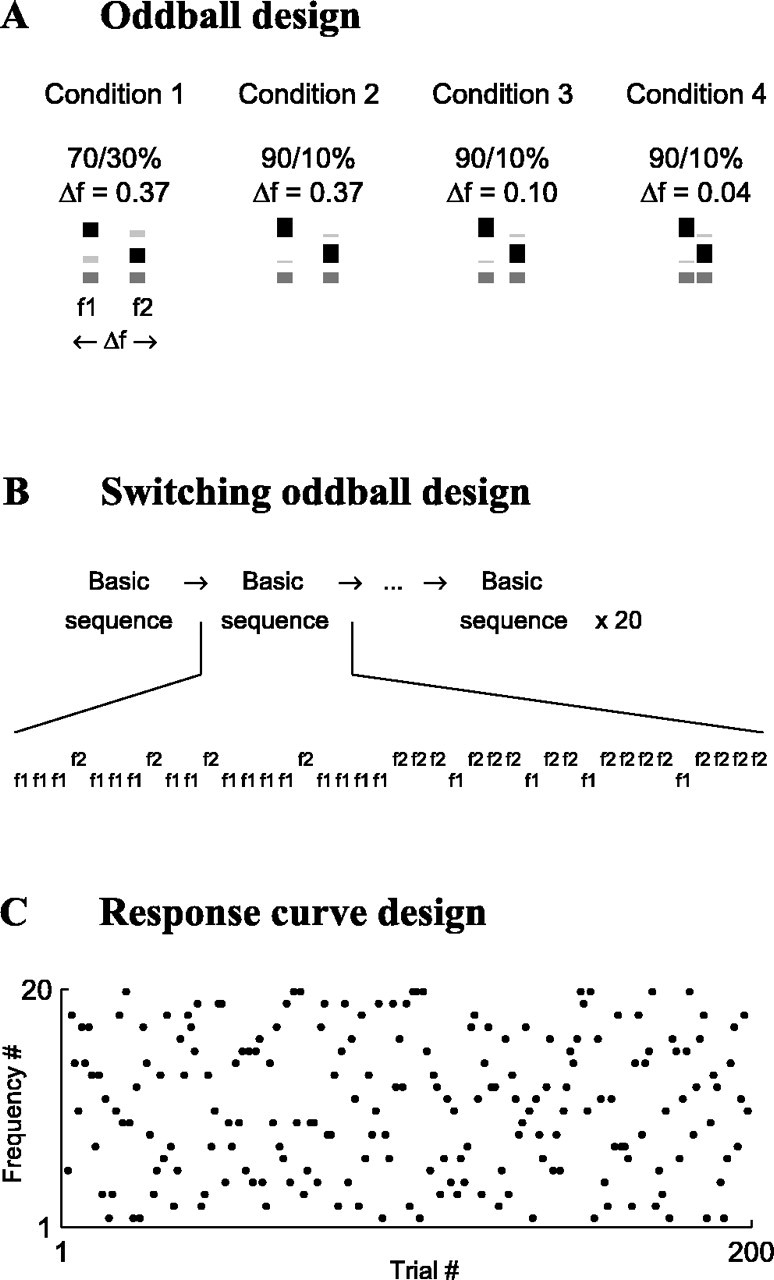
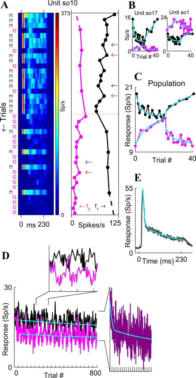
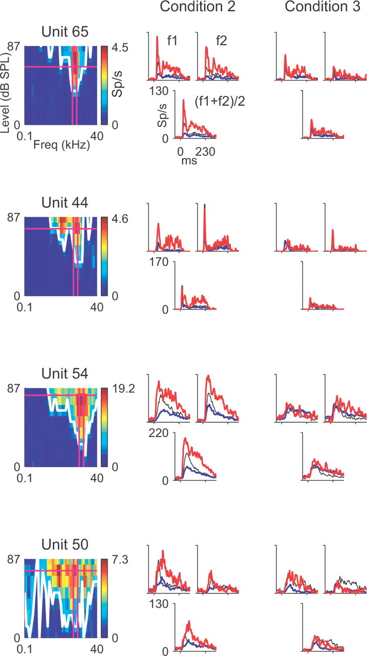
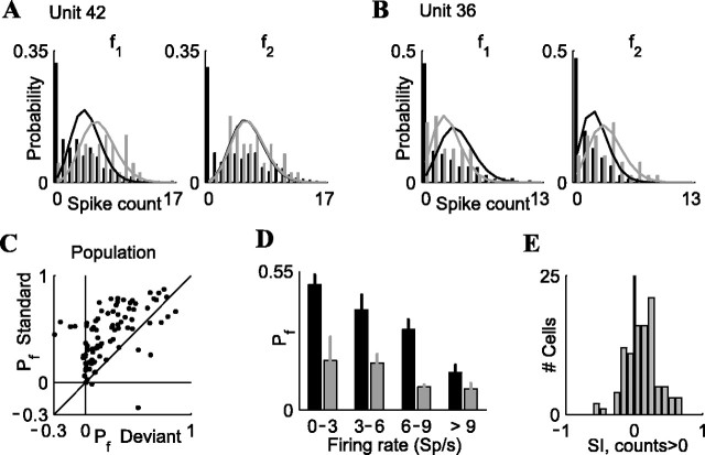
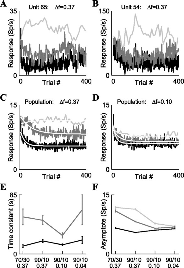
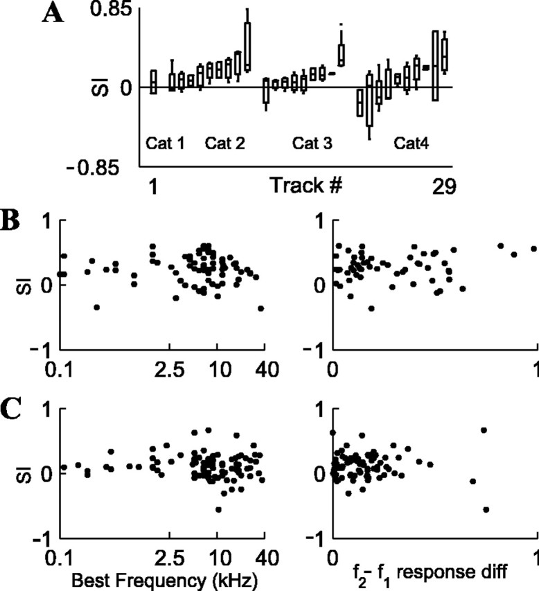
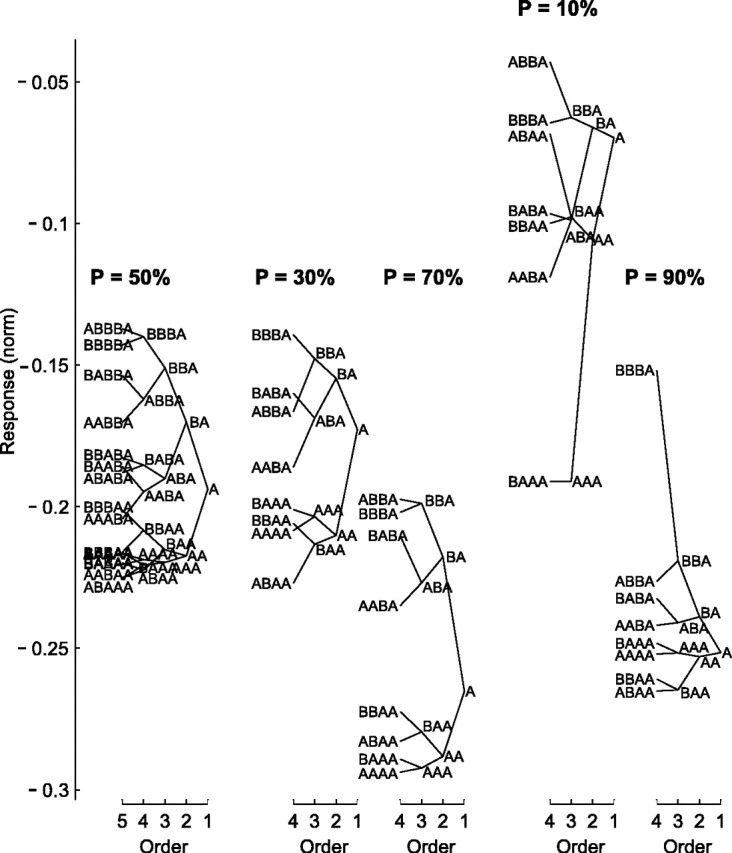
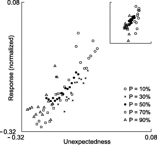
Neurons in primary auditory cortex (A1) of cats show strong stimulus-specific adaptation (SSA). In probabilistic settings, in which one stimulus is common and another is rare, responses to common sounds adapt more strongly than responses to rare sounds. This SSA could be a correlate of auditory sensory memory at the level of single A1 neurons. Here we studied adaptation in A1 neurons, using three different probabilistic designs. We showed that SSA has several time scales concurrently, spanning many orders of magnitude, from hundreds of milliseconds to tens of seconds. Similar time scales are known for the auditory memory span of humans, as measured both psychophysically and using evoked potentials. A simple model, with linear dependence on both short-term and long-term stimulus history, provided a good fit to A1 responses. Auditory thalamus neurons did not show SSA, and their responses were poorly fitted by the same model. In addition, SSA increased the proportion of failures in the responses of A1 neurons to the adapting stimulus. Finally, SSA caused a bias in the neuronal responses to unbiased stimuli, enhancing the responses to eccentric stimuli. Therefore, we propose that a major function of SSA in A1 neurons is to encode auditory sensory memory on multiple time scales. This SSA might play a role in stream segregation and in binding of auditory objects over many time scales, a property that is crucial for processing of natural auditory scenes in cats and of speech and music in humans.

Figure 1.

Auditory stimuli used in this study. A, The oddball design: stimuli consisted of sequences of standard and deviant tones, differing in frequency. We used three probability ratios (p = 90/10, 70/30, and 50/50%) and three frequency differences (Δf = 0.37, 0.10, and 0.04), and their combination defined four stimulus conditions. For each condition, we schematically represent here the three blocks that were used. The stimulus probability is denoted by the height of bars as well as by their darkness (standard, black; deviant, light gray; 50/50% control, dark gray), and the frequency difference Δf is denoted by the horizontal separation. B, The switching-oddball design, consisting of a basic 40 trial sequence, in which the f₁/f₂ probability ratio switched in the middle from 80/20 to 20/80% (Δf = 0.37). This frozen basic sequence, which is given at the bottom, was repeated 20 times for a total of 800 trials and was identical for all neurons. C, The response-curve design. We randomly presented 20 frequencies, 10 repetitions each, spanning a total frequency range of 0.97 octaves (each dot represents 1 stimulus trial).

Figure 6.

Time course of adaptation to frozen switching-oddball stimuli, showing multiple time scales of adaptation (n = 24 neurons in A1). A, Left, Responses of a single neuron to the two tones that comprise the basic 40 trial stimulus sequence (the sequence is displayed along the ordinate) (see also Fig. 1 B). The responses were averaged over the 20 repetitions of this frozen sequence and are represented as color-coded PSTHs. Right, Spikes counts for the same cell, for frequencies f₁ (black) and f₂ (magenta). Arrows mark examples of predeviant (blue) and postdeviant (red) standards. B, Average responses of two more neurons as a function of the sequential position of the stimulus within the basic 40 stimulus sequence (black, f₁; magenta, f₂), together with exponential fits (cyan). C, Exponential fits to the population mean responses (same colors as in B). We computed the mean response over all neurons and then used nonlinear least-squares fitting of exponential functions to this mean. D, Population responses to the full 800 trials, unfolding the 20 repetitions of the basic sequence (ticks at the bottom). Top inset, “Zoom in” on the responses to three consecutive repetitions of the basic sequence. Right inset, Average population response to frequencies f₁ and f₂, with separate exponential fits for trials 1-80 (steep cyan curve), for which we used the exponential computed from the p = 50% responses in Figure 5C (τ = 48.4 sec), and for trials 81-800 (shallow cyan curve). E, Mean within-tone population response in the switching-oddball design, averaged over the two frequencies for all of the trials and all neurons (gray), together with a double-exponential fit (cyan).

Figure 2.

Activity of four neurons in A1 in response to the oddball stimuli. Each row corresponds to one neuron. First column, FRA (color coded) with the tuning curve (white line) and amplitude and frequencies used for the oddball stimuli (magenta; vertical lines are for Δf = 0.37). Second column, Responses to condition 2 of the oddball stimuli (p = 90/10%; Δf = 0.37), for frequency f₁ and f₂ separately, as well as the mean response to f₁ and f₂. Third column, Responses to condition 3 (p = 90/10%; Δf = 0.10). Colors denote standard (blue), deviant (red), and p = 50% control (black). The stronger response to the deviant than to the standard (red > blue), both when f₁ was the deviant and f₂ was the deviant, demonstrates the presence of SSA.

Figure 4.

Adaptation increases the proportion of failures in the responses of A1 neurons. A, B, Spike-count distributions for two neurons (A, B), for frequencies f₁ and f₂, when they were standards (black bars) or deviants (gray bars). Solid lines, Fits of Poisson distributions, based on non-zero counts only. C, The parameter p_f indicates the observed probability of zero-counts minus predicted probability from the Poisson fits, plotted for standards against deviants. D, More failures for standards than for deviants. Population means of p_f for standards and deviants, grouped by firing rate, are shown. Note that each neuron contributes twice to this plot; for example, for the deviant it may contribute to a high firing-rate bin and for the standard it may contribute to a lower firing-rate bin. Number of neurons averaged for each bar, from left to right: 57, 38, 13, 21, 11, 6, 16, and 32. E, Adaptation index SI, computed for non-zero counts only. Data are for stimulus condition 2 (p = 90/10%; Δf = 0.37).

Figure 5.

Time course of adaptation to oddball stimuli in A1 neurons. A, B, Two examples of adaptation to stimulus condition 2 (90/10%; Δf = 0.37), plotted separately for deviant (light gray), p = 50% (medium gray), and standard (black). Responses were smoothed with a three-element hamming window for display only. C, Time course of adaptation of the mean population responses for stimulus condition 2 (90/10%; Δf = 0.37); colors are the same as in A and B. The abscissa shows the average serial position of the trial inside the block; the ordinate shows the mean population firing rate (without any smoothing) together with single-exponential fits (white). D, Time course of adaptation of the mean population responses for stimulus condition 3 (90/10%; Δf = 0.10). E, Time constants of fitted exponentials for the four stimulus conditions (data for deviants are not shown because the weak adaptation made computation of these time constants very inaccurate). F, Asymptotic firing rates of the exponential fits. In all population panels, for each of the four stimulus conditions, we used all of the neurons presented with this condition: n = 30, 99, 107, and 68, respectively, for conditions 1-4 (the 4 stimulus conditions are listed from left to right in E, F).

Figure 3.

A, Adaptation columns in A1: box plots of SI values for neurons recorded along the same electrode track (29 tracks from 4 cats), sorted for each cat in ascending order of average SI. Each box plot represents the median, interquartile range, and total range of SIs along a single electrode track. Only electrode tracks with two neurons or more are shown (total n = 91 neurons). In cat 1, only a single track was recorded (track #1). Data are for p = 90/10%; Δf = 0.10. B, No correlation between the SI and the BF of the neuron (left; n = 76 neurons) or the f₂ - f₁ response difference (right; n = 56) for p = 90/10%, Δf = 0.37. C, Same lack of correlation for p = 90/10%, Δf = 0.10 (n = 90 and 81 for left and right panels, respectively).

Figure 7.

Local history trees for the responses to the oddball stimuli, for Δf = 0.37, computed separately for each of the five stimulus probabilities (p = 10, 30, 50, 70, and 90%). Ordinate, Mean normalized response to a stimulus, grouped according to the preceding stimulus sequence, starting from the stimulus (A) and ending with fourth-order sequences (e.g., BBBA) (see Results). The fifth-order sequences (e.g., BBBBA), were much less orderly and therefore were drawn only for p = 50% for illustration. Each sequence in the tree connects with two higher-order sequences (corresponding to the addition of B or A before that sequence) and one lower-order sequence. All of the plotted sequences are based on averaging of at least 25 repetitions among all trials × all neurons (the AAAA sequence for p = 10% did not meet this criterion and therefore was omitted). Trees for p = 50, 10, and 90% are based on 68 neurons; trees for p = 30 and 70% are based on 29 neurons.

Figure 8.

Fitting a linear model of stimulus “unexpectedness” to A1 responses. Each dot represents the mean population response to one fifth-order local sequence, with symbol shape representing the global probability p. Main plot, Δf = 0.37. Inset, Δf = 0.10 (x-axis and y-axis limits: -0.31 to -0.12).

Figure 9.

Dynamics of the fits to the linear model of Figure 8, computed using a 50 msec sliding window. The windows were shifted by 20 msec (before and after the stimulus), 10 msec (during the stimulus), or 5 msec (during the onset responses). The abscissa denotes the centers of the 50 msec bins. The vertical lines indicate time of stimulus offset (t = 230 msec). A, Regression slopes of the model, separately for the global probability p (black) and local sequence M (dark gray). Light gray, Difference between the population response to the deviant and the standard, DS = PSTH(Deviant) - PSTH(Standard), inverted and scaled. Inset, Scaling of all three curves to the same minimum. B, Fraction of variance explained by the model R². Inset, “Zoom in” on the initial time. C, Fraction of variance explained by the model, R², showing separately the significant time bins (filled circles and solid lines) and nonsignificant time bins (empty circles and dotted lines). Light gray, DS = PSTH(Deviant) - PSTH(Standard). Inset, Scaling all three curves to the same maximum.

Figure 10.

No adaptation in auditory thalamus (MGB; n = 27 neurons; p = 90/10%; Δf = 0.10). A, Time course of mean population responses to the oddball stimuli, showing no decline over trials (gray, deviant; black, standard) (compare Fig. 5D). Data for p = 50% were not plotted here, because of the smaller number of neurons (n = 17). B, Local history trees (compare Fig. 7). C, The linear model of stimulus “unexpectedness” provides a poor fit to MGB responses (compare Fig. 8). In both B and C, some dots were missing for the p = 10% and p = 90% conditions, because not all possible sequences occurred in the data.

Figure 11.

Adaptation-induced bias in neuronal response curves measured over a narrowband range of 0.97 octaves (A1; n = 89 neurons). A, Response-curve design (see also Fig. 1C). Stimuli were tones of 20 frequencies × 10 repetitions each, totaling 200 trials (dot raster illustrates the first 40 trials). Gray circles, Trials preceding the occurrences of frequency 10 (denoted by arrow). At frequency 10, the near trials (□) and the far trials (×) are marked separately (see Results for definitions). U-shaped curve, Theoretical average frequency difference (AFD) of each tone from the preceding trials. B, Three neurons in primary auditory cortex, showing for each neuron the far (light gray), full (dark gray), and near (black) response curves and the full - far difference curve (plotted below each graph). Error bars represent SEM, averaged across frequencies. Gray rectangles indicate spontaneous firing rate ± SD. C, Mean population responses for neurons with an average full firing rate of more than five spikes per second (Sp/s) (n = 42). D, Difference curve of the population responses (black), overlaid with the U-shaped average frequency difference curve (gray), demonstrating the U-shaped bias in narrowband response curves. Main plot, Full - far (n = 42 neurons); left inset, near - far (n = 42); right inset: full - far for all of the neurons (n = 89). Error bars, SEM y-axis limits for left and right insets: -7.5-1.5 and -2.25-0.45 spikes/sec, respectively. E, Scatter plot of bias index versus adaptation index. Histograms, Index distributions, together with numbers of neurons above and below 0 (black lines).

References

1. Abbott LF, Varela JA, Sen K, Nelson SB (1997) Synaptic depression and cortical gain control. Science 275: 220-224. - PubMed
1. Bar-Yosef O, Rotman Y, Nelken I (2002) Responses of neurons in cat primary auditory cortex to bird chirps: effects of temporal and spectral context. J Neurosci 22: 8619-8632. - PMC - PubMed
1. Best AR, Wilson DA (2004) Coordinate synaptic mechanisms contributing to olfactory cortical adaptation. J Neurosci 24: 652-660. - PMC - PubMed
1. Bottcher-Gandor C, Ullsperger P (1992) Mismatch negativity in event-related potentials to auditory stimuli as a function of varying interstimulus interval. Psychophysiology 29: 546-550. - PubMed
1. Bregman AS (1990) Auditory scene analysis: the perceptual organization of sound. Cambridge, MA: MIT.
Publication types